Kirchhoff’s Circuit Laws: A Practical Guide for Real-World Electrical Analysis

If you’ve ever stared at a circuit diagram and caught yourself thinking, “Wait… where on earth is all this current going?”, you’re in good company. Even seasoned engineers have moments where a network feels more like a puzzle than a system. And honestly, that’s exactly why Kirchhoff’s circuit laws have survived since the 1840s. They give us the kind of clarity that cuts straight through the confusion.

The funny thing is, these laws aren’t complicated. They’re almost… obvious—once you hear them. But the power they offer? That’s where things get interesting. Knowing how to use them can save you hours of troubleshooting, help you size components with confidence, and make all those seemingly tangled circuits suddenly fall into place.

Before we dive deep, let’s warm up with a friendly, beginner-level overview.

What Are Kirchhoff’s Circuit Laws? (Beginner-Friendly Overview)

Kirchhoff’s circuit laws are considered as the fundamental circuit analysis laws and theorems. But don’t get mistaken, these laws are still used even if we use more advanced circuit analysis laws and theorems.

Kirchhoff’s laws were introduced first by a German physicist, Gustav Kirchhoff in 1845. These laws summarized the research of Georg Ohm and James Clerk Maxwell.

Kirchhoff’s laws are introduced to overcome the difficulty of using only Ohm’s law to analyze a circuit. Solving a circuit with multiple voltage or current sources will cost us a lot of time just to collect all the equations.

Leaving aside the strong point of Kirchhoff’s circuit laws, we will still use Ohm’s law to solve the equations we got from Kirchhoff’s laws.

There are few points and terms you need to understand before studying and mastering Kirchhoff’s circuit laws; they are branches, nodes, and loops. You can learn them first before continuing your study here if you haven’t had enough understanding.

The Kirchhoff circuit law is divided into:

• Kirchhoff’s current law
• Kirchhoff’s voltage law

With these two, without a doubt we can solve a complex electrical circuit even with multiple junctions, voltage or current sources, and even bridge networks.

Kirchhoff’s laws are flexible because we can use these in frequency and time domain.

You’ll see two ideas repeated throughout this article, and they’re surprisingly down-to-earth:

• Electric charge doesn’t vanish, and
• Energy doesn’t magically appear or disappear

From those two facts, we get the two famous laws: one for currents and one for voltages. If you’re just starting out, think of them as the “traffic rules” for circuits. They tell you how electrical flow behaves at intersections (nodes) and around paths (loops).

Why do these laws matter?

A few reasons come up right away:

• They let you analyze circuits that are too messy for simple series–parallel shortcuts.
• They’re the backbone of nodal analysis, mesh analysis, and even tools like SPICE.
• They work in DC and AC circuits, including phasor-based systems used in power engineering.
• They’re consistent with the assumptions inside standards like IEC 60364, IEEE 141, and the NEC.

Once you get comfortable with these laws, circuit analysis becomes less of a chore and more of a logical exercise. For now we will analyze a DC circuit.

Understanding Kirchhoff’s Current Law (KCL)

Kirchhoff’s current law is often called

• Kirchhoff’s first law
• Kirchhoff’s junction rule
• Kirchhoff’s nodal rule, and
• Kirchhoff’s point rule.

Let’s start with something intuitive: currents meeting at a node. You might catch yourself asking, “What are Kirchhoff’s circuit laws actually telling me here?”

Definition of KCL

Kirchhoff’s first law is based on the law of conservation of charge that requires that the algebraic sum of charge within a system cannot change.

Kirchhoff’s current law (KCL) says:

The sum of currents entering a node must equal the sum of currents leaving it.

And yes, it really is just that simple. No current gets stuck in the node, and none is lost. If 5 amps flow in from one branch and 3 amps leave through one branch, then 2 amps must leave through the others. It’s all about conservation of charge.

KCL Formula

The mathematical equation of KCL is

$$
\begin{align*}
\sum_{n=1}^N i_n=0
\end{align*}
$$

where :

\( N \) = number of branches which connected to the node

\( i_n \) = the nth current entering or leaving the node

With this law, currents entering a node can be assumed as positive, while the leaving currents as negative or vice versa.

In order to prove KCL, a set of currents \( i_k(t), k = 1,2,…,n \) , flow into a node, the algebraic sum of current at that node is

\( i_T(t) = i_1(t) + i_2(t) + i_3(t)+ … \)

Integrating both sides of the equation above makes

\( q_T(t) = q_1(t) + q_2(t) + q_3(t)+ … \)

Where

\( q_k(t)=\int_{}^{} i_k(t) dt \)

And

\( q_T(t)=\int_{}^{} i_T(t) dt \)

But the law of conservation of electric charge requires an algebraic sum of electric charges at the node must not change.

Thus,

\( q_T(t) = 0 \rightarrow i_T(t) = 0 \)

confirming the validity of KCL.

Please observe the illustration below to understand how KCL works.

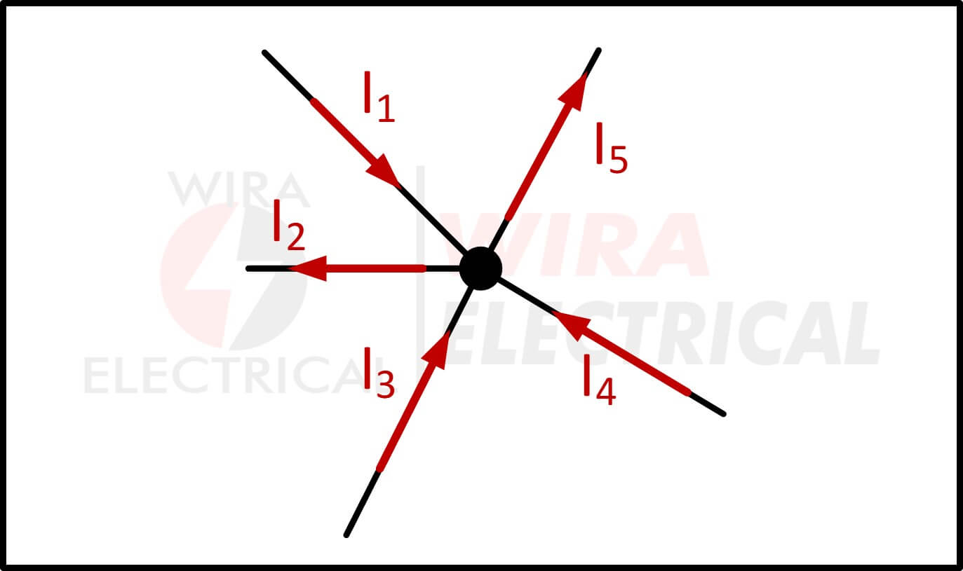
As we have read,

Kirchhoff’s current laws (KCL) states that the algebraic sum of currents entering a node (or a closed boundary) is zero.

Assuming the entering currents have positive sign and leaving currents have negative sign, then

\( I_1 + (-I_2) + I_3 + I_4 + (-I_5) = 0 \)

Furthermore, we can rewrite the equation above into

\( I_{\mbox{entering}} = I_{\mbox{leaving}} \)

Where

\(I_1 + I_3 + I_4 = I_2 + I_5 \)

We can conclude the alternative form of KCL as

The KCL equation is the sum of currents entering a node is equal to the currents leaving that node.

For easier explanation, let us imagine some current sources connected together in parallel. The combined current is the algebraic sum of the current supplied by individual sources.

Then, this example can be seen in the circuit below.

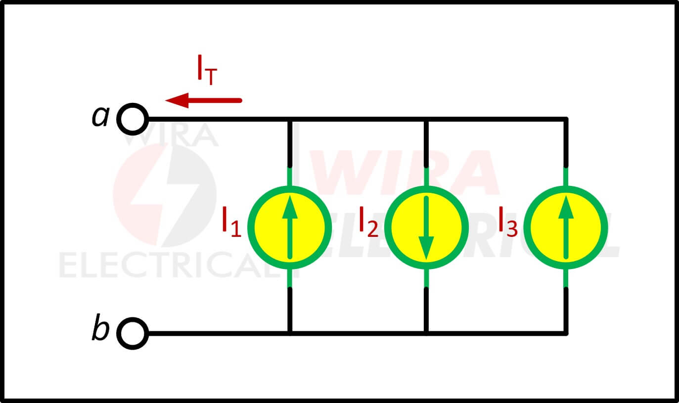
The combined or equivalent current source can be found by applying KCL to node a.

\( I_T = I_1 – I_2 + I_3 \)

and then combined to make a connection as seen below

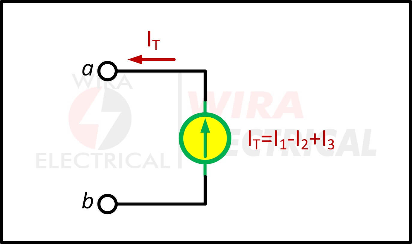
A circuit cannot contain two different current I1 and I2 in series unless I1 = I2.

KCL in AC systems

In AC analysis, per IEEE Std 1459, currents are treated as phasors:

\( \sum \widetilde{I} = 0 \)

The rule itself doesn’t change; you’re just working with complex numbers. This becomes important when analyzing industrial loads, especially those with non-unity power factors.

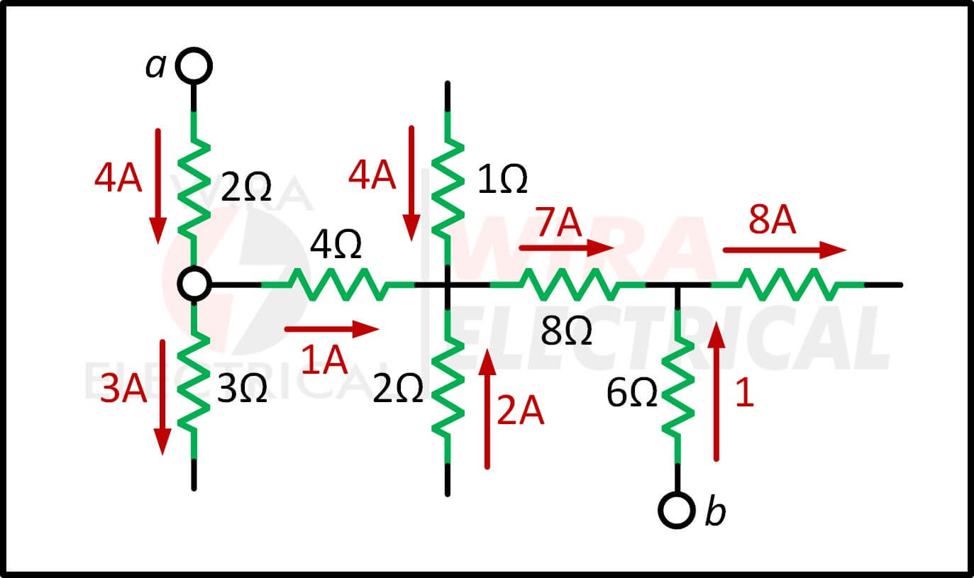
Kirchhoff’s Current Law Example

For an example, find the value of \( i \) in the circuit below:

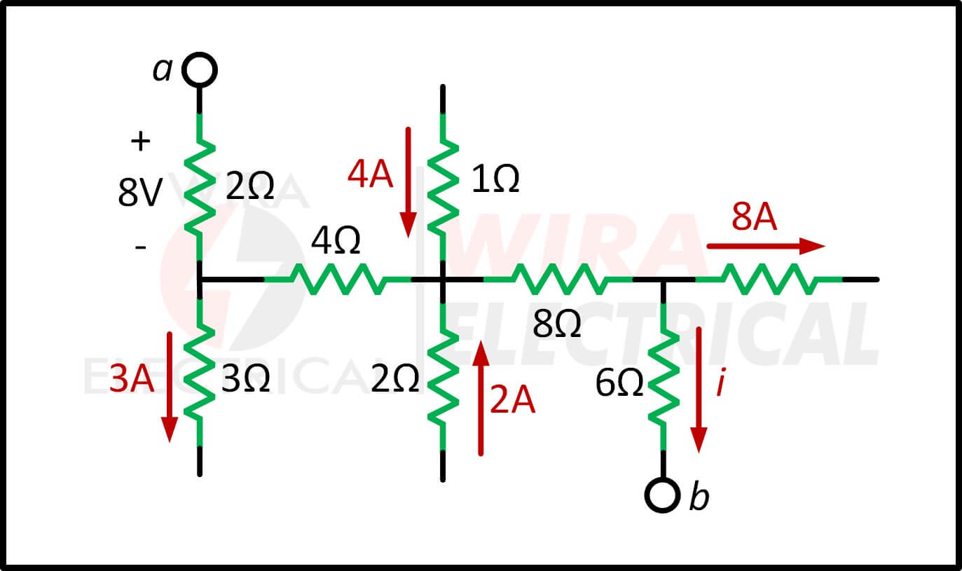
We can calculate the current leaving the point a ( \( I \) ) using Ohm’s law:

\( I = \frac{V}{R} = \frac{8}{2} = 4A \)

The current is entering the resistor because the positive sign of the 2Ω resistor is facing the point \( a \). Thus, the circuit becomes

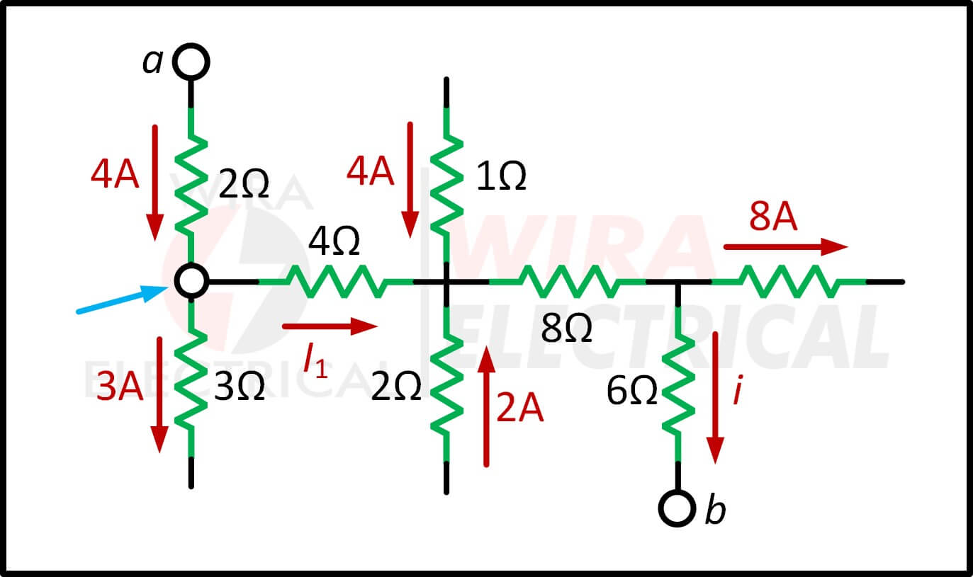
Assume that entering currents are positive, otherwise negative. Then,

\( 4 = 3 + I_1 \rightarrow  I_1 = 1A \)

Now we need to find \( I_2 \),

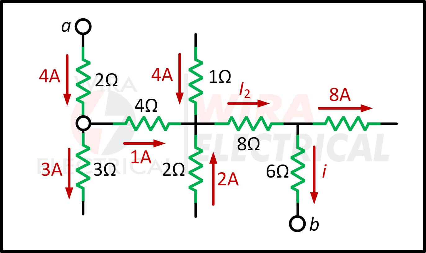
The value of \( I2 \) is

\( 1+4+2=I_2 \rightarrow  I_2 = 7A \)

From this circuit, we have every variable we need to solve the question.

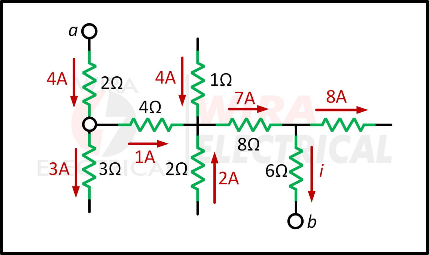
The value of i is

\( 7 = i + 8 \rightarrow  i = -1A \)

The negative value shows that the current should be in the opposite direction. Then

Understanding Kirchhoff’s Voltage Law (KVL)

If KCL is about charge, KVL is about energy—and honestly, this one feels even more intuitive once you see it in action.

Kirchhoff’s voltage law is often called:

• Kirchhoff’s second law,
• Kirchhoff’s second rule,
• Kirchhoff’s mesh rule, and
• Kirchhoff’s loop rule.

Definition of KVL

Kirchhoff’s second law is based on the principle of conservation of energy.

Kirchhoff’s voltage law (KVL) says:

The sum of all voltages around a closed loop must be zero.

The principle of Conservation of Energy means: if the current is moving in a closed-loop, it will reach the point where it started in the first place.

Hence, the initial potential has no voltage drop in the loop. Summary, the voltage drop in a loop is equal to the voltage sources met in the way.

It is important to pay attention to the quantity signs (positive and negative) of the circuit element.

If we write the equation with the wrong signs of the circuit element voltage drop, the calculation can be wrong.

Before moving on, let us learn what voltage drop is first.

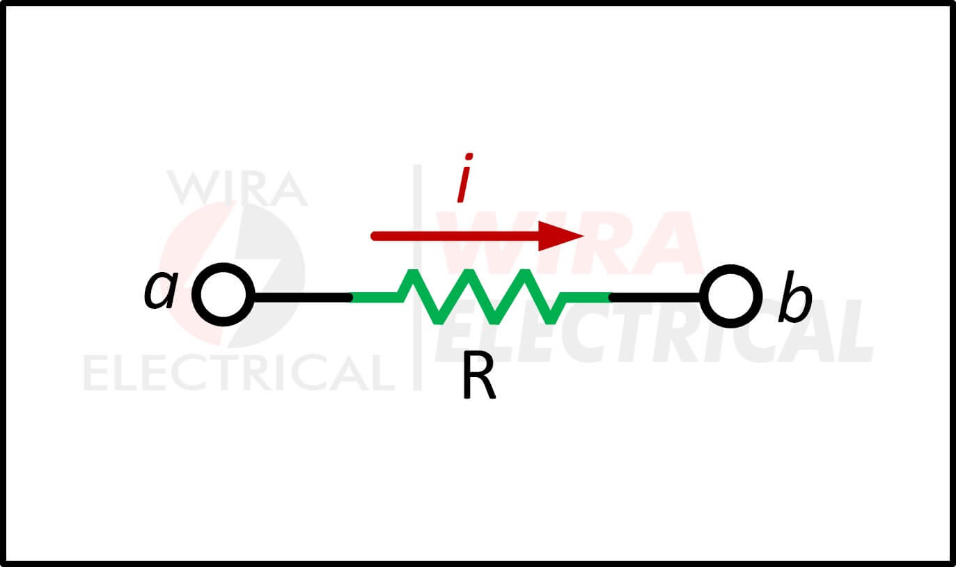
Above is the example of voltage drop for a single element. We will use a resistor here for easier explanation.

Let’s say the current I is the same with the positive charge flowing direction, from the left to the right (A to B).

We can say the current is flowing from the positive terminal to the negative terminal.

Because we are using the same direction as the same as the current direction, there will be a drop across the resistor.

The value of the voltage drop will be ( \( -iR \) ).

For the best step, we will pay attention to the polarity direction. The polarity sign of the element will follow the flow direction of the current through it.

Just decide the current flow in clockwise or counterclockwise before starting to write the equation.

Both of them will provide the correct answer, even if the result is in negative signs (it means the current is flowing in the opposite direction).

KVL Formula

\( \sum V = 0 \)

Again, pick a direction—clockwise or counterclockwise—and stick with it.

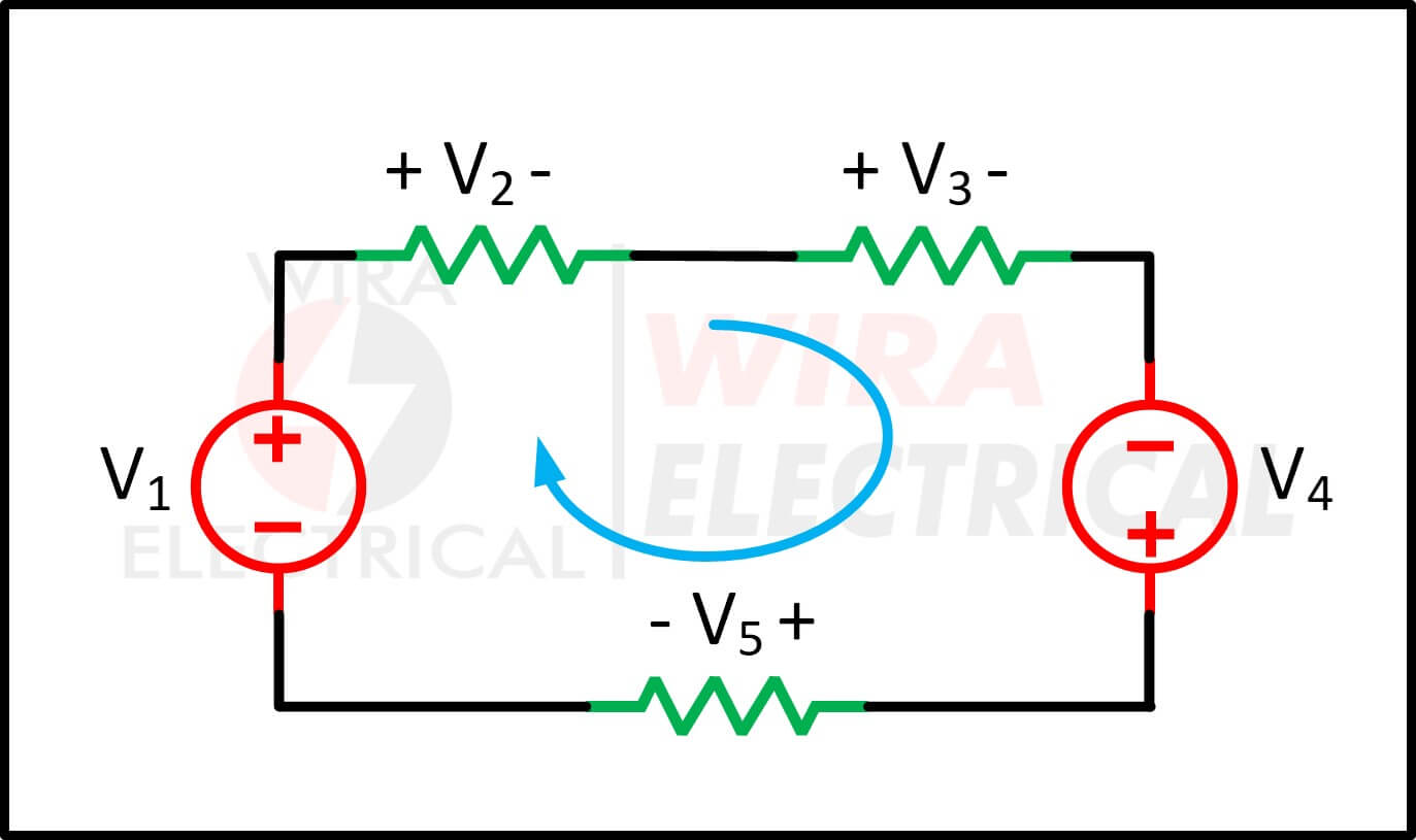
For better understanding, please take a look at the circuit below.

With the mathematical equation, KVL states

$$
\begin{align*}
\sum_{m=1}^M v_m=0
\end{align*}
$$

where \( M \) is the number of voltages in the loop (or the number of branches in the loop) and \( v_m \) is the \( m_{th} \) voltage.

The sign on each voltage is the polarity of the terminal encountered first as we travel around the loop.

So, we can start with any branch and go around the loop either in a clockwise direction or counterclockwise.

Assume we start with a clockwise direction then the voltages would be \( –v_1, +v_2, +v_3, –v_4, and +v_5 \) in order.

Hence the KVL yields

\( -v_1 + v_2 + v_3 – v_4 + v_5 = 0 \)

Rearranging equation gives

\( v_2 + v_3 + v_5 = v_1 + v_4 \)

Which may be interpreted as

\( \sum \mbox{Voltage drops} = \sum \mbox{Voltage rises} \)

For example for the voltage sources in the circuit below.

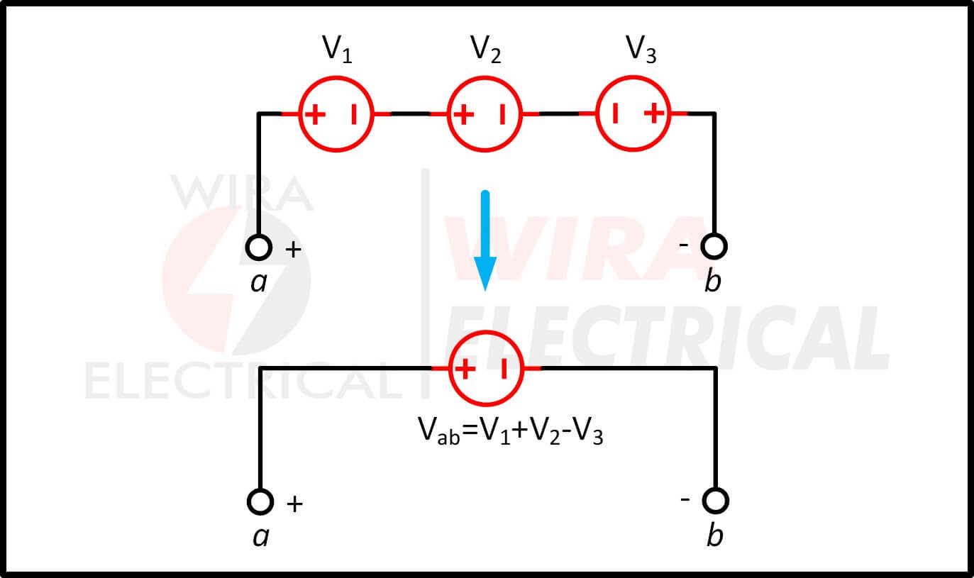
The combined or equivalent voltage source in the circuit above is obtained by using the KVL equation.

$$
\begin{align*}
-V_{ab} + V_1 + V_2 – V_3 = 0 \\
V_{ab} = V_1 + V_2 – V_3
\end{align*}
$$

Using two different voltages in parallel is violating KVL unless the values are the same.

Kirchhoff’s laws will take part on:

• Wye-Delta transformation
• Nodal analysis
• Mesh analysis

In AC circuits

KVL still holds, except voltages become phasors:

\( \sum \widetilde{V} = 0 \)

This is crucial when evaluating impedance networks, harmonic conditions, or power electronic loops.

Kirchhoff’s Current Law Example

For better understanding, observe the circuit below

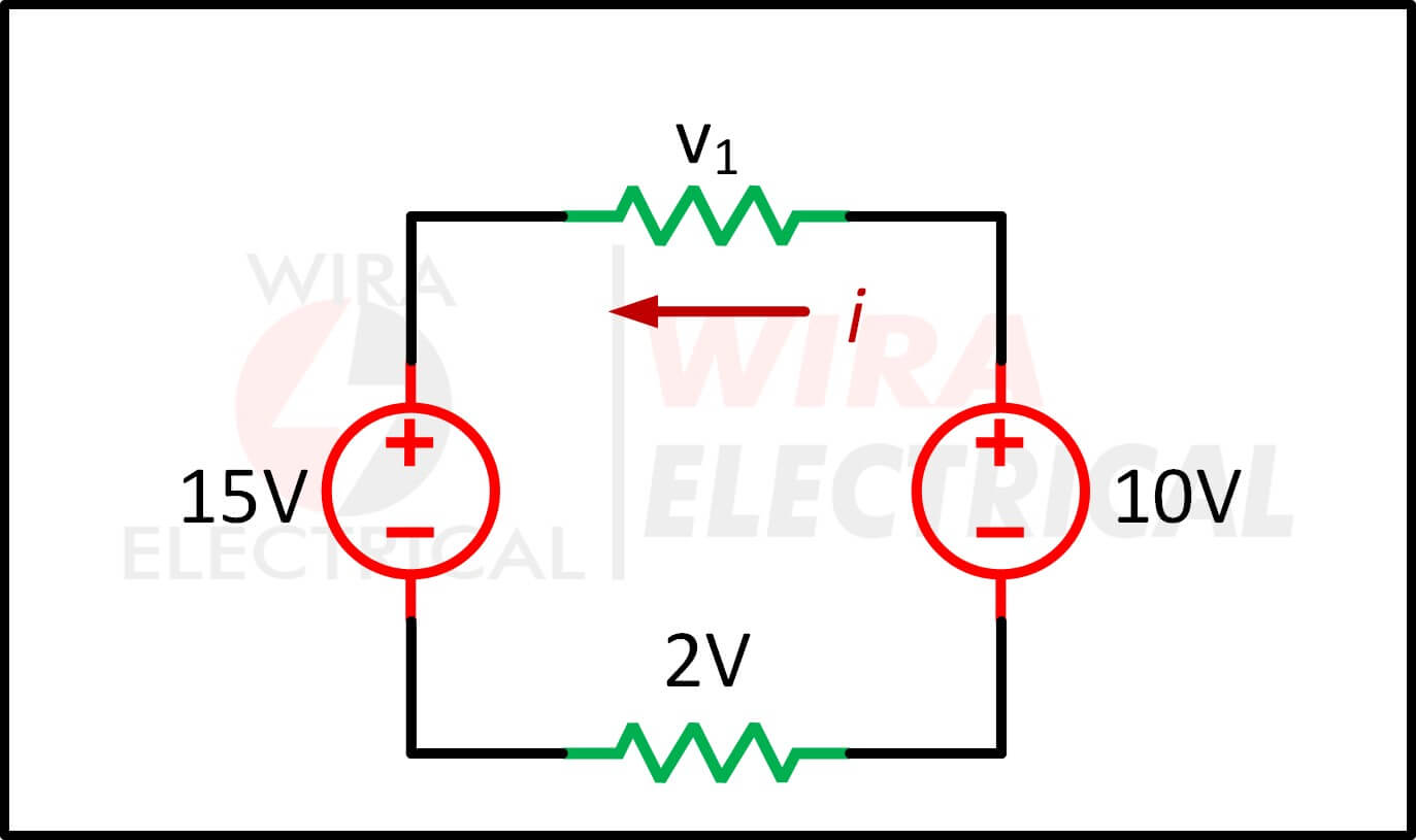
Since the current arrow indicator facing left, the loop should be counterclockwise. The positive sign of the upper resistor is on the right, and on the left for the bottom resistor. The resistance values in this circuit are ignored.

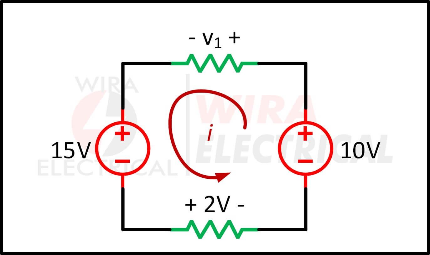
The KVL equation states that the algebraic sum of all voltages around a closed path (or loop) is zero. Then,

$$
\begin{align*}
\sum v &= 0 \\
v_1 + 15 + 2 – 10 &= 0 \\
v_1 &= -7V
\end{align*}
$$

The negative value indicates that the positive sign of the upper resistor should be on the left side and the current is in clockwise direction to make it have a positive value.

Kirchhoff’s Rules in Circuit Analysis

Once you’ve got a feel for KCL and KVL, you can combine them into structured methods. Engineers use these approaches every day—especially when circuits get complicated enough that mental math won’t cut it.

Nodal Analysis Using Kirchhoff Laws

This method leans on KCL.

The usual steps go like this:

1. Pick a ground node (usually the most connected one).
2. Assign voltages to the remaining nodes.
3. Apply KCL: the sum of currents leaving each node is zero.
4. Use Ohm’s Law to express each current.
5. Solve the resulting equations.

Nodal analysis shines when a circuit has lots of parallel paths. If you see branches everywhere, this is the method to reach for.

Mesh Analysis Using Kirchhoff’s Laws

Mesh analysis works with KVL.

Here’s the general rhythm:

1. Identify loops that don’t contain smaller loops inside them.
2. Assign a mesh current to each loop.
3. Apply KVL to each loop.
4. Write voltage drops in terms of mesh currents.
5. Solve the system of equations.

Mesh analysis is perfect when a diagram looks like it’s made of several rings connected together. Fewer nodes and more loops? Mesh analysis usually wins.

Key Formulas and Parameters You’ll Use

A quick table to keep your head clear:

Concept	Formula	Purpose
KCL	\( \sum I = 0 \)	Keeps charge balanced at any node
KVL	\( \sum V = 0 \)	Ensures energy conservation in a loop
Ohm’s Law	\( V = I R \)	Helps convert between current and voltage
Power	\( P = V I \)	Useful for checking compliance with NEC/IEC
Impedance	\( \widetilde{Z} = R + jX \)	Essential for AC and phasor analysis

These aren’t just formulas—they’re the backbone of virtually every steady-state circuit analysis method.

Step-by-Step Example: Using Kirchhoff’s Laws to Solve a Circuit

Let’s try a straightforward example. It’s one thing to read definitions, but applying them is where everything “clicks.”

Example Circuit Setup

Suppose you’ve got:

• A 12 V DC source
• \( R_1 = 4 \Omega \) 
• \( R_2 = 6 \Omega \) 
• \( R_3 = 12 \Omega \) connected from the middle node to ground

This is the kind of circuit you might bump into in a simple sensor interface or a basic power divider.

Step 1 — Assign currents

Let currents be:

• \( I_1 \)​ through \( R_1 \)​
• \( I_2 \)​ through \( R_2 \)
• \( I_3 \) through \( R_3 \)

Step 2 — Apply KCL at the node

\( I_1 = I_2 + I_3 \)

Pretty standard.

Step 3 — Use Ohm’s Law to express the currents

Define the node voltage as \( V_x \) :

\( I_1 = \frac{12-V_x}{4}, I_2 = \frac{V_x}{6}, I_3 = \frac{V_x}{12} \)

Step 4 — Substitute and solve

​\( \frac{12-V_x}{4}=\frac{V_x}{6}+\frac{V_x}{12} \)

Solving this gives:

\( V_x = 7.2V \)

And the currents:

\( I_1 = 1.2 A, I_2 = 1.2A, I_3 = 0.6 A \)

This is one of those Kirchhoff laws example problems where everything feels surprisingly neat when you get to the final numbers.

Real-World Applications of Kirchhoff’s Laws

These laws aren’t textbook trivia—they’re part of everyday engineering work.

Power Distribution and Protection

You’ll use KCL and KVL in:

• Neutral current calculations in three-phase systems
• Load-balancing studies
• Short-circuit current evaluations
• Compliance checks with IEC 60364, IEEE 141, and NEC 220

Electronics and PCB Design

From transistor biasing to filter design, these laws show up everywhere.

They help you understand:

• Feedback loops in amplifiers
• ADC input networks
• Sensor interfaces
• Voltage divider behavior with non-ideal loading

Industrial Automation

If you’ve worked with 4–20 mA loops, PLC modules, or industrial signal conditioners, you’ve applied Kirchhoff without even thinking about it.

Power Electronics

Converters, inverters, and rectifiers all rely on KVL/KCL for modeling. Even harmonic analysis uses the same principles—just dressed up in phasor math.

Advantages & Disadvantages of Kirchhoff’s Laws

A quick comparison:

Category	Advantages	Drawbacks
Simplicity	Intuitive and universal	Manual math can get long
Accuracy	Works in AC and DC	Assumes lumped components
Flexibility	Applies to any topology	Not ideal for nonlinear devices
Standards	Aligned with IEC/IEEE models	Struggles with RF parasitics

Tips, Best Practices & Common Mistakes

This section might save you some headaches.

Best Practices

• Pick your current directions early and stick to them—even if you guess.
• Annotate diagrams aggressively; engineers who label everything make fewer mistakes.
• Use KCL for circuits with many branches, and KVL when loops dominate.
• In AC circuits, treat impedance carefully—one wrong sign in reactance will throw everything off.
• Cross-check with power calculations to verify that your numbers make physical sense.

Common Mistakes

• Flipping current directions mid-calculation
• Forgetting the effect of controlled sources
• Ignoring parasitics in high-frequency applications
• Assuming KVL works in systems with significant mutual inductance

A note on limitations

Kirchhoff’s laws limitations show up mainly in:

• RF and microwave circuits
• Long transmission lines (where distributed models apply)
• Circuits with strong magnetic coupling
• Systems operating near resonances

In those cases, Maxwell’s equations give a more accurate picture.

Kirchhoff’s Laws Limitations

Kirchhoff’s laws may be considered as the simplest circuit analysis. But, they have their own limitations depending on the type of the circuit.

Below are the limitations of Kirchhoff’s laws:

• KCL is used with the assumption that the current is only flowing in wires and conductors. But, it will be different if we analyze High-Frequency circuits, where the parasitic capacitance can’t be ignored anymore.
• For some cases, currents can flow in an open circuit because conductors and wires are acting as transmission lines.
• KVL is used with the assumption that there is no fluctuating magnetic field linking to the closed-loop. While the presence of changing magnetic fields in a High-Frequency circuit but short-wavelength AC circuit, the electric field is not a conservative vector field.
• Electric field and EMF could be induced and cause the KVL breaks.
• In a transmission line, the electric charge changes over time and violates the KCL.

Conclusion

If you’ve stuck with me until now, you’ve walked through the same reasoning that many professional engineers use daily. Kirchhoff’s circuit laws aren’t fancy, but they’re incredibly dependable. They sit right at the center of circuit analysis—steady, predictable, and surprisingly elegant once you get comfortable with them.

Whether you’re troubleshooting a misbehaving PCB or validating load calculations in a low-voltage panel, these laws help you think clearly. Tools can automate the math, sure, but understanding the principles lets you spot errors, challenge assumptions, and build smarter designs.

In short: learn these laws well, and they’ll pay you back throughout your entire engineering career.

Frequently Asked Questions (FAQ)

References

• IEC 60364 – Low Voltage Electrical Installations
• IEEE Std 141 (Red Book)
• NEC (NFPA 70)
• IEEE Std 1459 – Definitions for AC Power
• Alexander & Sadiku — Fundamentals of Electric Circuits
• Dorf & Svoboda — Introduction to Electric Circuits