What Is Mesh Current Analysis, Really?

Mesh current analysis is used to analyze an electric circuit using the flowing currents in a closed loop of a circuit. Even though we already have Ohm’s law and Kirchhoff’s laws, those two give us more math equations to be solved. Mesh Current Analysis or Maxwell’s Circulating Currents or Loop Current Method is able to lessen the number of equations greatly.

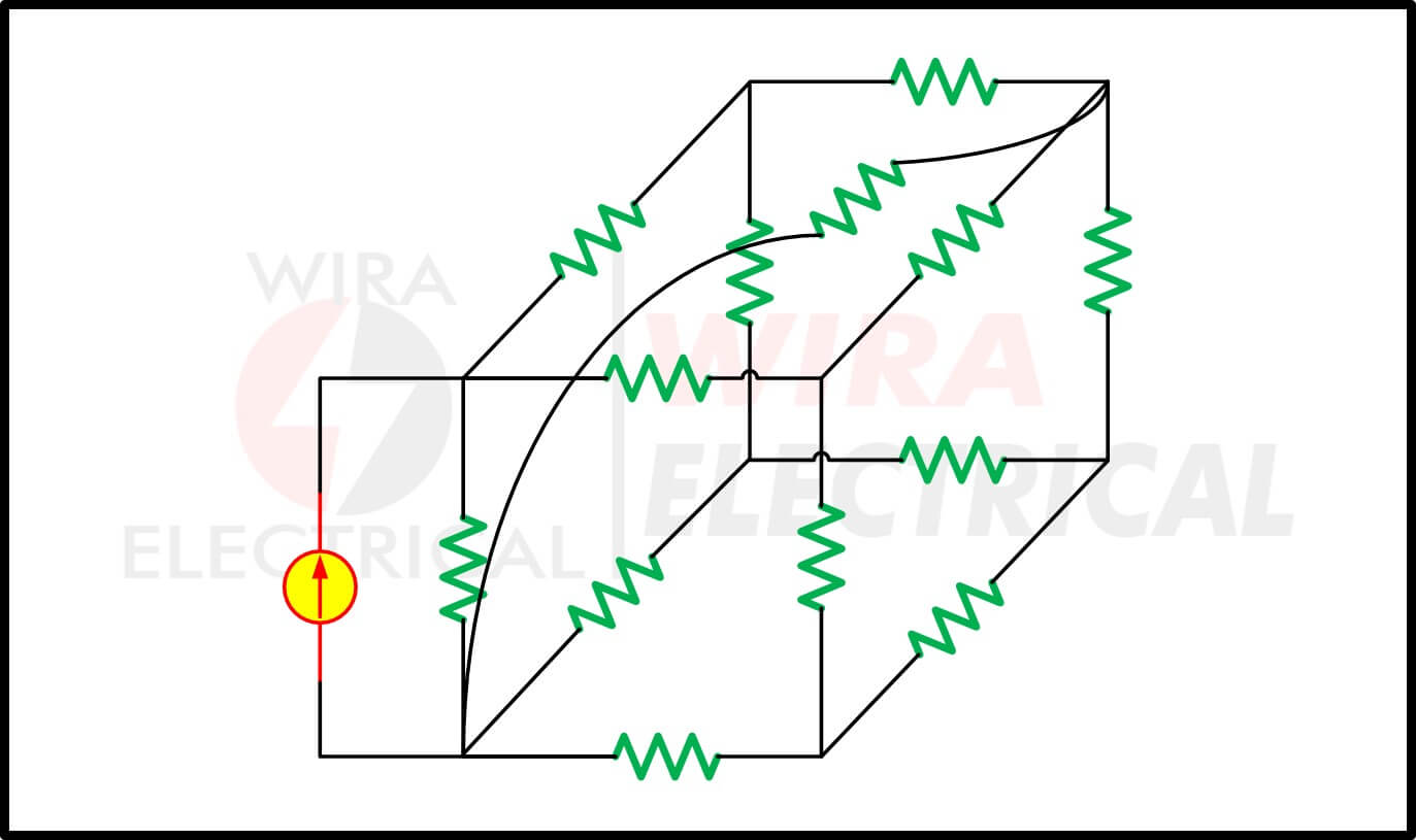
Keep in mind: mesh current analysis can only be used in the planar circuit. What is a planar circuit anyway? It is a circuit that can be redrawn with no branches crossing one another, otherwise, the non planar circuit can be seen below.

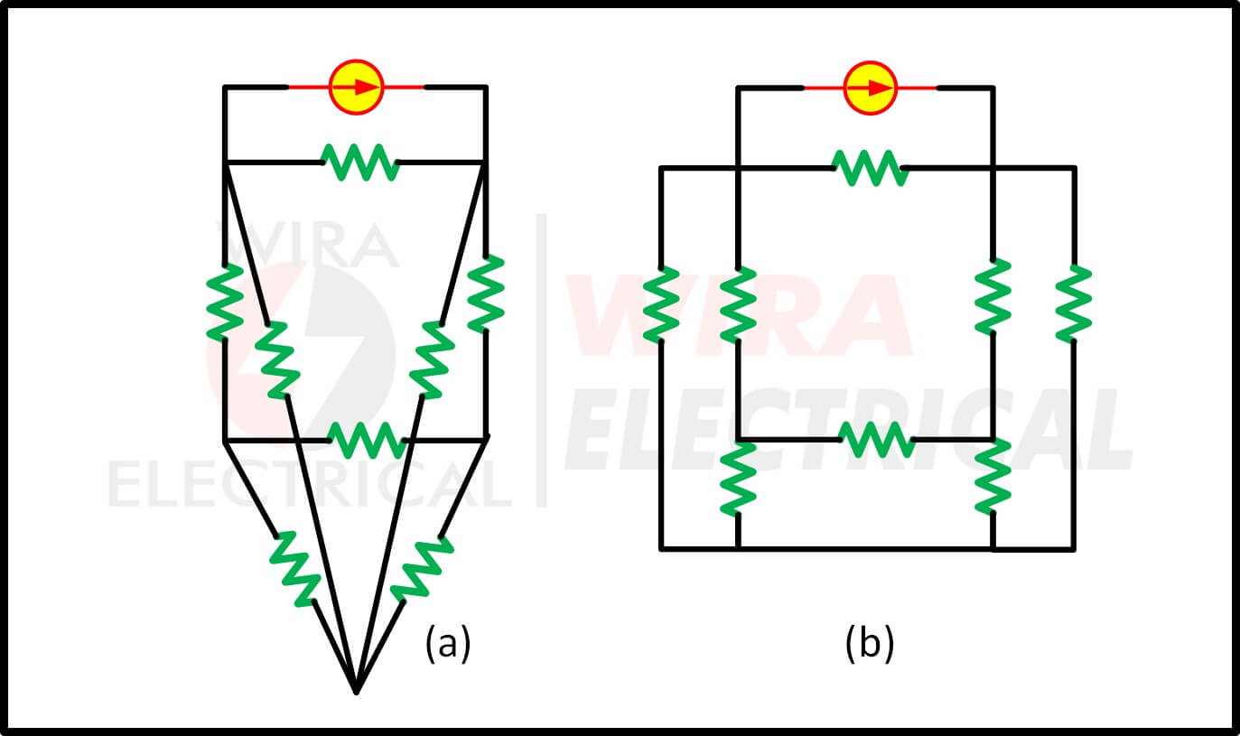
A circuit may have crossing branches and still be planar if it can be redrawn such that it has no crossing branches like shown below.

What is Loop and Mesh

We need to completely understand the term of the mesh since we will mention it every time we use this mesh current method. Mesh is basically an ‘exceptional’ loop. I am sure you are well aware of what is a loop in an electrical circuit.

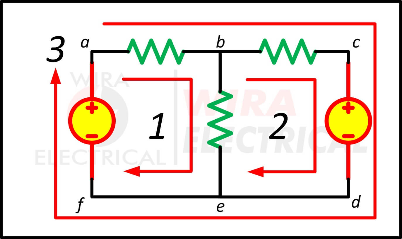
For comparison, take notice of the 3 loop dc circuit below:

Let’s refresh that now, what is a loop in an electrical circuit?

Loop is formed by a set of nodes. If the current flows from a starting node and passes through a set of nodes without passing the same node twice, it means the current flows in one loop.

The figure above is clear that the circuit has 3 loops, labelled by clockwise arrows 1, 2, and 3. But, do we also have three meshes? That’s the question right there.

Don’t get fooled by the representation of the arrows in the circuit since both loop and mesh are represented by clockwise or counterclockwise arrows.

Mesh generally has the same meaning as a loop, but a mesh is a loop without a loop inside it.

The difference didn’t hit you? Then take note below,

A mesh is a loop which does not contain any other loops within it.

We don’t need further explanation. From the circuit above only loop 1 and loop 2 are considered as meshes because loop 3 is containing other loops (loop 1 and 2). Hence in that circuit we have three loops (1, 2, and 3) and two meshes (1 and 2).

In that circuit, the paths abefa and bcdeb are meshes, but path abcdefa is not a mesh.

Like we read earlier, the current flowing through a mesh or closed-loop is known as mesh current. We will satisfy KVL in every condition when using mesh analysis.

For better and easier understanding, we will forbid the use of the current circuit in mesh analysis this time for a planar circuit. This does not mean mesh analysis is only limited to a voltage source. You will know why down here.

In the mesh analysis of a circuit with n meshes, we use these three following steps.

Steps to Determine Mesh Currents:

1. Assign mesh currents i₁, i₂, …., in to the n meshes.
2. Apply KVL to each of the n meshes. Use Ohm’s law to express the voltages in terms of the mesh currents.
3. Solve the resulting n simultaneous equations to get the mesh currents.

How to Mesh Current Analysis

Let’s proceed with the mesh current method. We will use the circuit above. We will assign the voltage sources and resistors with labels as shown below:

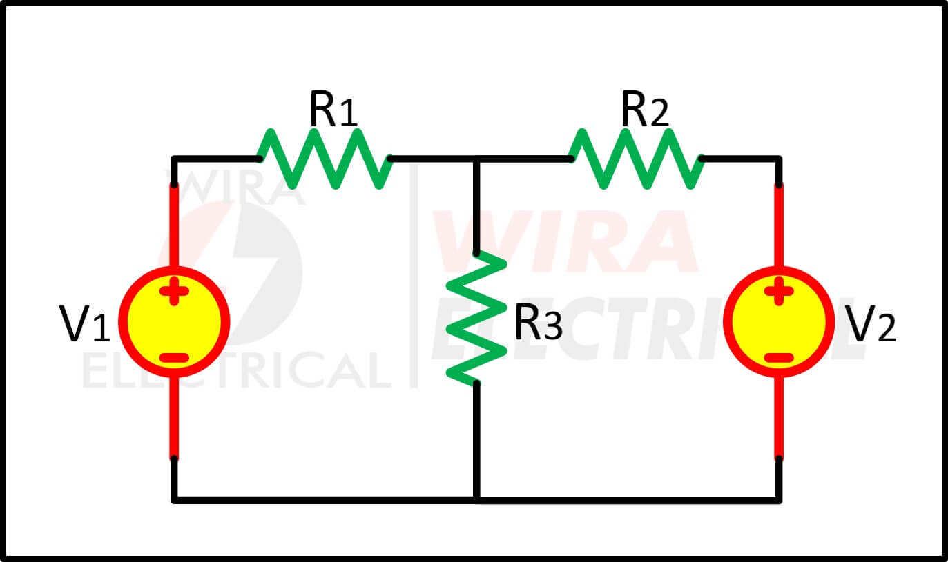
And then we apply the meshes with the clockwise direction and then we assign the labels to the currents and polarity for the resistors. Remember that we assign positive polarity to the resistor’s terminal entered by the current for the first time. Because the R₃ is in intersection between meshes 1 and 2, we assign i₃ to it for now.

We will get the following equations as below:

For mesh 1 (i₁):

\begin{align*}
(i_{1}R_{1})+(i_{3}R_{3})-V_{1}= 0
\end{align*}

For mesh 2 (i₂):

\begin{align*}
(i_{2}R_{2})+V_{2}+(i_{3}R_{3})= 0
\end{align*}

And those are the equations for two meshes we have. But how do we solve 3 unknown variables with only 2 equations?

The answer is: THIS WILL BE HARD

But to make things easier, we can write i₃ with another equation.

How? Check the mesh current analysis procedure below:

Mesh Current Analysis Procedure

For those of you who haven’t learned the mesh current analysis or want to refresh your memory, we will learn it now step-by-step carefully. Not to make things complicated after reading the explanation above, we will still use the circuit above as an example with known variable values.

Mesh analysis current directions

First, we determine the current directions for each mesh. It is up to you whether they are in clockwise or counterclockwise directions or a mix of them. We will go in a clockwise direction now.

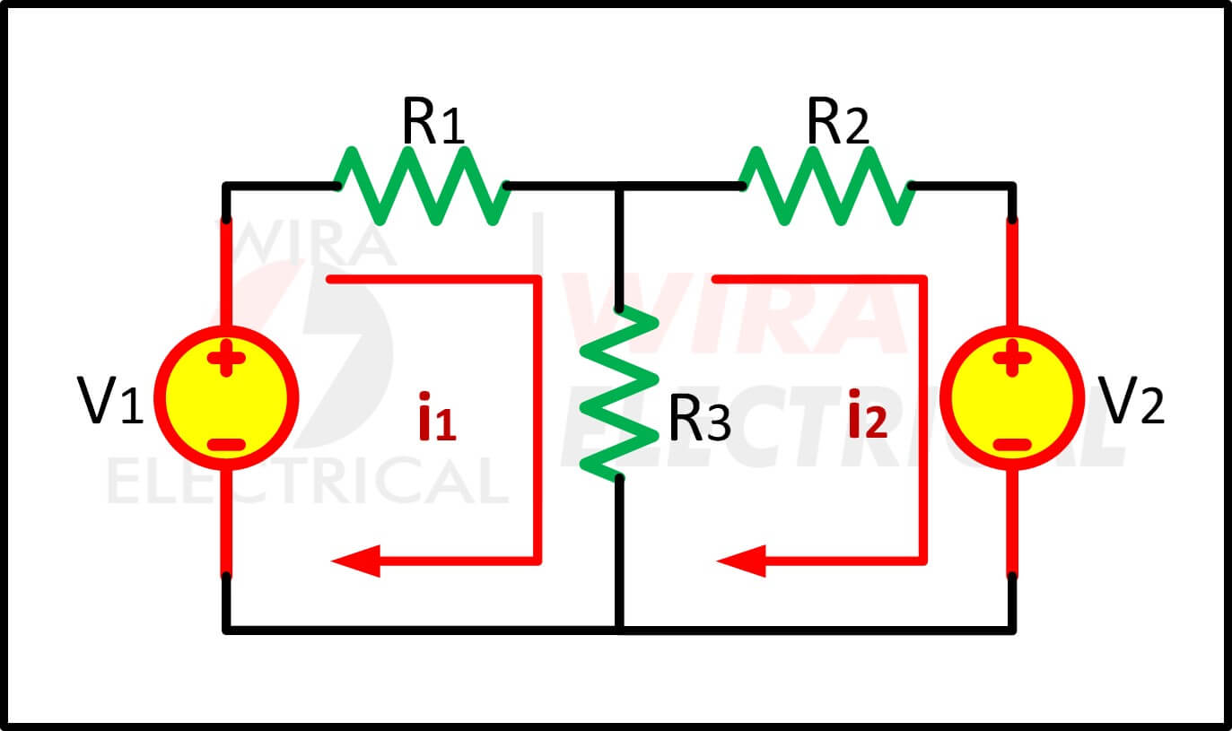
Labelling the circuit elements

We now label all the circuit elements with positive and negative polarity depending on the current direction using passive sign convention. For the currents passing the R₃, it depends on which mesh we are analyzing at the moment. Below you will find the explanation.

Find the KVL mesh equations

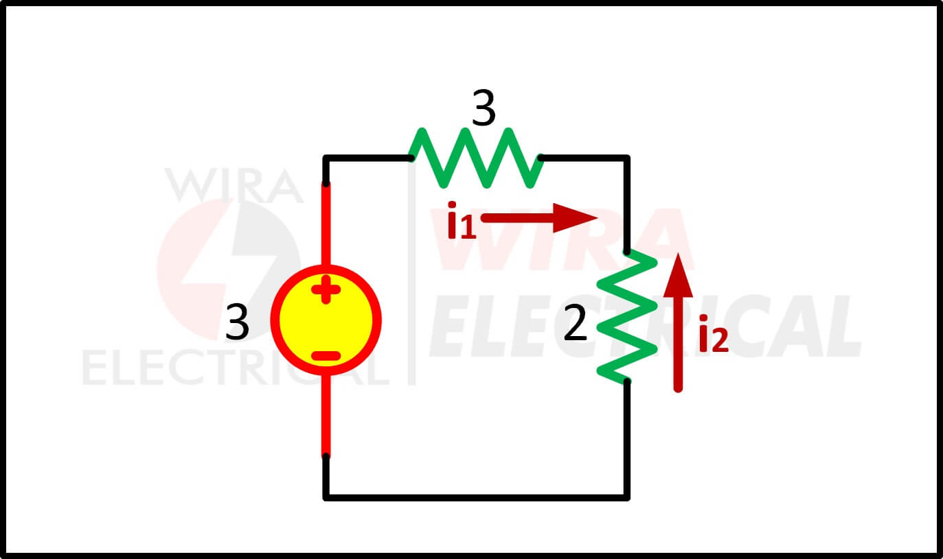
We will write down all the KVL equations to solve the circuit. But before that let’s give the numbers for each variable we have. The final circuit will be:

We will use a clockwise direction for each mesh.

For mesh 1,

We get:

\begin{align*}
-V_{1}+i_{1}R_{1}+(i_{1}-i_{2})R_{3}&=0\\
-3+3i_{1}+2(i_{1}-i_{2})&=0\\
3i_{1}+2i_{1}-2i_{2}&=3\\
5i_{1}-2i_{2}&=3
\end{align*}

The value of V₁ = -3 because the mesh 1 is entering the voltage source terminal from its negative polarity.

For mesh 2,

We get:

\begin{align*}
i_{2}R_{2}+V_{2}+(i_{2}-i_{1})R_{3}&=0\\
4i_{2}+5+2(i_{2}-i_{1})&=0\\
4i_{2}+2i_{2}-2i_{1}&=-5\\
2i_{1}-6i_{2}&=-5
\end{align*}

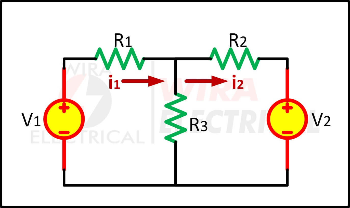
If you are still confused about the currents entering the R₃, assume we are analyzing the mesh 1. If we analyze mesh 1, we will prioritize the i₁. Look at the figure below.

For mesh 1, the sum of the currents entering the R₃ will be

\begin{align*}
V_{R3}=(i_{1}-i_{2})R_{3}
\end{align*}

If we analyze the mesh 2,

\begin{align*}
V_{R3}=(i_{2}-i_{1})R_{3}
\end{align*}

Now we have ‘2’ equations for ‘2’ meshes.

For mesh 1,

\begin{align*}
5i_{1}-2i_{2}=3
\end{align*}

For mesh 2,

\begin{align*}
2i_{1}-6i_{2}=5
\end{align*}

Solve the KVL mesh equations

As stated before, for every ‘n’ meshes there will be ‘n’ KVL equations. We have:

\begin{align*}
5i_{1}-2i_{2}=3\rightarrow \mbox{mesh 1}\\
2i_{1}-6i_{2}=5\rightarrow \mbox{mesh 2}
\end{align*}

We change the mesh 1 equation into:

\begin{align*}
5i_{1}-2i_{2}&=3\\
-2i_{2}&=3-5i_{1}\\
i_{2}&=\frac{5i_{1}-3}{2}
\end{align*}

Substituting this into the mesh 2 equation,

\begin{align*}
2i_{1}-6i_{2}&=5\\
2i_{1}-6(\frac{5i_{1}-3}{2})&=5\\
2i_{1}-15i_{1}+9&=5\\
-13i_{1}&=-4\\i_{1}&=0.3077
\end{align*}

Substituting i₁ into mesh 1 equation,

\begin{align*}
5i_{1}-2i_{2}&=3\\
5(0.3077)-2i_{2}&=3\\
1.5385-2i_{2}&=3\\
i_{2}&=-0.73075
\end{align*}

It means the direction of i₂ is counterclockwise 0.73075 A. With the current values have been discovered, you can find other variables you desire.

Mesh Current Analysis with Current Source

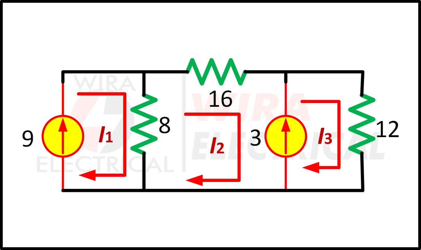
The example above is the mesh analysis with the voltage source. Now we will analyze a circuit with current sources. It will not be that different from the voltage source, but indeed we need to know the step difference. For example, we will use the circuit below:

We have to find the value of i.

First, we assign the mesh current,

We now write down all the KVL equations. We will get 3 equations since there are 3 meshes in the circuit.

For mesh I₁,

\begin{align*}
i_{1}=9
\end{align*}

Why do we have value without any effort? Because in mesh 1 there is a current source without any intersection with another mesh current.

For mesh I₂ and I₃,

\begin{align*}
I_{3}-I_{2}&=3\\
I_{3}&=3+I_{2}
\end{align*}

When there is a current source in an intersect branch, we call this circuit a supermesh. The depth of supermesh will be explained in the next post about Supermesh Analysis.

From supermesh:

\begin{align*}
8(I_{2}-I_{1})+16I_{2}+12I_{3}=0
\end{align*}

Substituting I₃ to this equation results

\begin{align*}
8(I_{2}-9)+16I_{2}+12(3+I_{2})&=0\\
8I_{2}-72+16I_{2}+36+12I_{2}&=0\\
36I_{2}&=36\\
I_{2}&=1A
\end{align*}

Hence,

\begin{align*}
i=I_{2}=1A
\end{align*}

Mesh Analysis 3 Loops

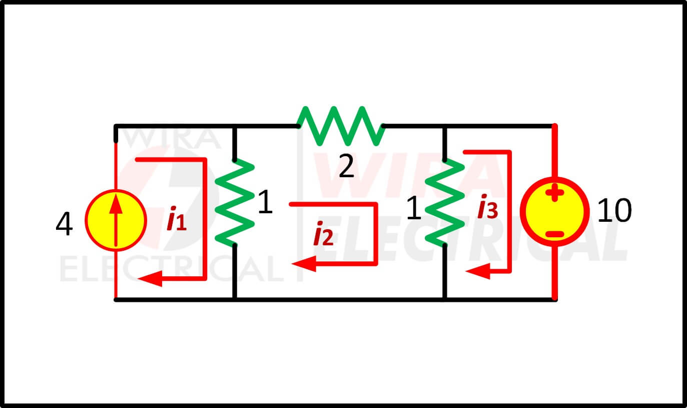
If a circuit has 3 meshes it will still be easy enough to solve as long as there is no current source in an intersection branch with another mesh current. The example below is the mesh analysis 3 loops with an only voltage source and current source in one mesh to make it easier.

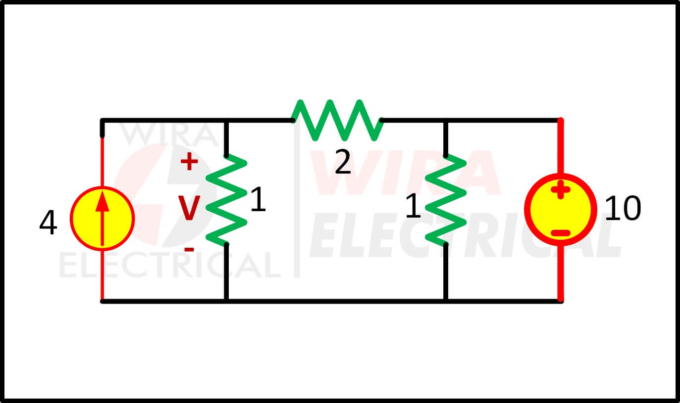
We assign the mesh current,

For mesh 1,

\begin{align*}
i_{1}=4A
\end{align*}

For mesh 2,

\begin{align*}
1(i_{2}-i_{1})+2i_{2}+1(i_{2}-i_{3})&=0\\
1(i_{2}-4)+2i_{2}+i_{2}-i_{3}&=0\\
-4+4i_{2}-i_{3}&=0\\
i_{3}&=4i_{2}-4
\end{align*}

For mesh 3,

\begin{align*}
1(i_{3}-i_{2})+10&=0\\i_{3}-i_{2}&=-10\\
i_{3}&=i_{2}-10
\end{align*}

Substituting mesh 3 equation into mesh 2,

\begin{align*}
i_{2}-10&=4i_{2}-4\\
3i_{2}&=-6\\
i_{2}&=-2A
\end{align*}

Now we have to find the V. The resistor is passed by the mesh current i₁ and i₂. Since the positive polarity is in top side,

\begin{align*}
V&=IR\\
V&=(i_{1}-i_{2})1\\
V&=(4-(-2))1\\
V&=6V
\end{align*}

Mesh Current Analysis Example

It is wise for us to analyze more circuits for better understanding. Let us study the examples below:

1. Find the branch currents value I₁, I₂, and I₃ of the circuit below using mesh analysis. Assume the mesh current directions for both loops are in the clockwise direction.

Answer:

First, we write down all the KVL equations. For two meshes we will get two equations:

For mesh 1,

\begin{align*}
-15+5i_{1}+10(i_{1}-i_{2})+10=0\\
3i_{1}-2i_{2}=1\tag{1.1}
\end{align*}

For mesh 2,

\begin{align*}
6i_{2}+4i_{2}+10(i_{2}-i_{1})-10=0\\
i_{1}=2i_{2}-1\tag{1.2}
\end{align*}

Using substitution,

Substitute (1.2) into (1.1) and we get

\begin{align*}
6i_{2}-3-2i_{2}=1\quad\Rightarrow\quad i_{2}=1A
\end{align*}

From (1.2) we get

\begin{align*}
i_{1}&=2i_{2}-1\\
&=2-1\\
&=1A
\end{align*}

Thus,

\begin{align*}
I_{1}&=i_{1}=1A\\
I_{2}&=i_{2}=1A\\
I_{3}&=i_{1}-i_{2}=0
\end{align*}

2. Find the value of i in circuit below using mesh analysis!

Let’s draw the mesh currents:

For mesh I₁,

\begin{align*}
-5+6I_{1}-5i_{a}&=0
\end{align*}

Where:

\begin{align*}
I_{1}=i_{a}
\end{align*}

Then

\begin{align*}
-5+6i_{a}-5i_{a}&=0\\
i_{a}&=5A
\end{align*}

For mesh I₂,

\begin{align*}
5i_{a}+10I_{2}+25&=0\\
25+10I_{2}+25&=0\\
I_{2}=\frac{-50}{10}&=-5A\\
i=-I_{2}=-(-5)&=5A
\end{align*}

Where Mesh Analysis Actually Shows Up in Practice

It’s easy to see this as a purely academic exercise. It isn’t.

Residential Ring Circuits

UK and Australian wiring standards use ring final circuits where power is delivered from both ends of a ring-shaped loop. This creates a genuine multi-mesh network. Engineers analyzing load distribution, cable sizing, and fault currents in ring mains apply loop current principles directly — the method maps cleanly onto the ring topology.

IEC 60364, which governs low-voltage electrical installations internationally, requires that cable ampacity not be exceeded under any loading condition, and mesh analysis is how you verify that.

PCB Power Delivery and EMI Analysis

In power electronics, every trace has resistance. Every loop in a PCB layout carries a mesh current, and when switching transients occur, those loops radiate. Engineers use mesh analysis — sometimes extended to include inductance — to model ground bounce, voltage ripple, and parasitic coupling between power rails.

IEC 61000 (the EMC standard family) sets conducted and radiated emission limits that only make sense to evaluate if you understand how current distributes across a board’s loop structure.

Industrial Control Panels and Fault Analysis

Multi-source industrial circuits — the kind you’d find feeding motor starters, VFDs, and lighting loads on the same bus — often have interconnected branches that can’t be analyzed with simple series-parallel reduction.

Mesh analysis gives you the fault current in each loop, which you need to properly size and coordinate overcurrent protection devices. NEC Article 240 and IEC 60947-2 both require selective coordination for main and branch circuit breakers — and that coordination analysis depends on knowing the loop currents under fault conditions.

Simulation Software Under the Hood

LTspice, Multisim, PSpice, MATLAB’s Simscape — all of them solve circuits using variants of modified nodal analysis (MNA), which is directly descended from mesh and nodal methods.

If you understand mesh analysis, you understand why simulators behave the way they do when they encounter degenerate circuits, convergence issues, or voltage source loops. That insight is genuinely valuable for debugging simulation models.

Nodal Analysis vs Mesh Analysis: An Honest Comparison

I’ve seen arguments about this in engineering forums that go on far longer than they should. Both methods work. The difference is efficiency — and occasionally, topology.

Here’s a side-by-side breakdown:

Factor	Mesh Current Analysis	Nodal Analysis
Theoretical basis	Kirchhoff’s Voltage Law (KVL)	Kirchhoff’s Current Law (KCL)
Solves for	Mesh (loop) currents	Node voltages
Number of equations	M (number of meshes)	N−1 (nodes minus reference)
Works on non-planar circuits?	No	Yes
Special case for current sources	Supermesh required	Straightforward — KCL handles directly
Special case for voltage sources	Straightforward — KVL handles directly	Supernode required
Preferred when…	Voltage sources dominate; M < N−1	Current sources dominate; N−1 < M
Common in…	Power loop analysis, ring circuits	Power system bus analysis, op-amp circuits

 The practical decision rule: count M (meshes) and N−1 (non-reference nodes). Use the method that gives you fewer equations. When they’re equal, pick whichever better matches the source types in the circuit.

One thing worth noting: experienced engineers often shift between methods mid-analysis. Mesh for one sub-circuit, nodal for another. There’s no rule against it once you know both well enough.

Advantages and Disadvantages: Being Honest About the Method

No technique is perfect for every situation. Here’s what mesh analysis does well — and where it has real limitations.

Where It Shines

• Fewer unknowns than branch-current analysis. Instead of solving for every individual branch current, you solve for M mesh currents. For dense circuits, that reduction is substantial.
• Structured and systematic. The setup process is almost algorithmic. That makes it easy to teach, easy to learn, and easy to verify.
• Matrix-friendly. The resistance matrix [R] for mesh analysis is always symmetric (for circuits with only resistors and independent sources), which makes it well-suited for numerical solvers.
• Efficient for voltage-source-dominant circuits. Voltage sources drop directly into the KVL right-hand side without complications.
• Power calculations are direct. Once you have mesh currents, power in any resistor is P = R × (branch current)², where branch current is trivially derived.

Where It Struggles

• Planar circuits only. This is the hard constraint. Non-planar topologies require a different approach.
• Current sources require extra steps. The supermesh technique is manageable, but it adds cognitive load, especially when there are multiple current sources.
• Mesh currents aren’t directly measurable. You can’t clip an ammeter around a mesh current. Every measurement requires a conversion step back to branch currents.
• More equations than nodal when M > N−1. In node-rich, mesh-sparse circuits, nodal analysis is strictly more efficient.
• Dependent sources complicate the setup. You need to express control variables in terms of mesh currents before writing equations, which requires careful bookkeeping.

Practical Tips and the Mistakes That Keep Showing Up

After working through a lot of these problems — and watching others work through them — the errors tend to cluster around a handful of recurring issues. Here are the ones that matter most.

Tips That Actually Help

• Be disciplined about consistent current direction. All clockwise, or all counterclockwise — pick one and stick with it for every mesh in the circuit. Mixed conventions are the single biggest source of sign errors.
• Mark shared branches before you write a single equation. Circle them, highlight them, put a star next to them. Any branch with two mesh currents flowing through it needs to be flagged before the algebra starts.
• Switch to matrix form at three or more meshes. Seriously. Trying to do substitution on three simultaneous equations by hand is tedious and error-prone. A 3×3 matrix takes thirty seconds to set up and makes the structure of the problem immediately visible.
• With dependent sources, define the control variable first. Write it explicitly in terms of mesh currents before you set up any KVL equation. This avoids the situation where you’re trying to handle the dependency mid-equation.
• Always verify. Not optional. Substitute your solved mesh currents back into every KVL equation and confirm it sums to zero. If it doesn’t, something is wrong in the setup — not necessarily in the arithmetic.

Common Mistakes (And Why They Happen)

• Wrong sign on shared-branch voltage drop. The drop across a shared resistor R is R×(I_own − I_adjacent), not R×I_own. Missing the subtraction is an extremely common error, especially when working quickly.
• Attempting KVL through a current source. You can’t. Current sources don’t have defined voltage drops — that’s the whole point. If you catch yourself writing a voltage term for a current source, stop and use the supermesh technique instead.
• Counting the outer boundary as a mesh. It’s not. The perimeter loop of the entire circuit encloses other loops, which disqualifies it as an independent mesh. Over-counting meshes gives you more equations than unknowns and leads to a contradictory system.
• Skipping the planarity check. Most practical circuits are planar. But occasionally a circuit schematic looks planar and isn’t — especially when wires are drawn to cross for routing convenience. Redraw if you’re unsure.
• Inconsistently applying the source sign rule. The sign of a voltage source in a mesh equation depends on whether it aids or opposes the assumed mesh current direction. Getting this wrong on even one source corrupts the entire equation for that mesh.

Wrapping Up: What You’ve Actually Learned Here

Mesh current analysis isn’t magic. It’s discipline. The whole technique rests on one physical law (KVL), one abstraction (mesh currents), and one systematic process (write one equation per mesh, solve, verify). None of that is complicated in isolation. What makes it powerful is that the structure scales — a two-mesh circuit and a six-mesh circuit are handled with exactly the same method, just more equations.

The real-world relevance is genuine. Ring circuit analysis under IEC 60364, fault current calculations required by NEC Article 240, EMC loop modeling per IEC 61000 — these aren’t hypothetical applications. They show up in engineering work on actual projects.

And the honest truth about the tricky parts: current sources aren’t as scary as they look once you understand the supermesh logic. Dependent sources take a bit more care, but the method handles them. Non-planar circuits are the only real boundary condition, and they’re rare in practice.

If you worked through the example in this guide and followed the steps, you already have the core skill. The rest is practice — getting faster at identifying shared branches, getting more comfortable with matrix setup, building the instinct for when to use mesh vs nodal. That comes with repetition, not with reading more explanations.

Thanks for sticking with this. Circuit analysis rewards patience, and the fact that you’re here working through it carefully puts you in better shape than most.

References

• Nilsson, J.W. & Riedel, S.A. (2019). Electric Circuits, 11th Edition. Pearson.
• Hayt, W.H., Kemmerly, J.E., & Durbin, S.M. (2018). Engineering Circuit Analysis, 9th Edition. McGraw-Hill.
• Alexander, C.K. & Sadiku, M.N.O. (2020). Fundamentals of Electric Circuits, 7th Edition. McGraw-Hill.
• IEEE Std 1459-2010: IEEE Standard Definitions for the Measurement of Electric Power Quantities Under Sinusoidal, Nonsinusoidal, Balanced, or Unbalanced Conditions.
• IEC 60364: Low-voltage electrical installations — applicable parts for ring circuit design and cable ampacity.
• IEC 61000: Electromagnetic Compatibility (EMC) — conducted and radiated emission standards.
• National Electrical Code (NEC) 2023, Article 240: Overcurrent Protection.
• IEC 60947-2: Low-voltage switchgear and controlgear — Circuit-breakers.

FAQ