Supernode Analysis Easy Solving

Picture this. You’re halfway through a nodal analysis problem, you’ve labeled your nodes, you’re about to write KCL — and then you notice a voltage source sitting directly between two non-reference nodes. Not between a node and ground. Between two actual nodes.

You try writing KCL at the first node. The current through the voltage source shows up as an unknown. You can’t express it with Ohm’s Law because there’s no resistance. You try the second node. Same problem. You’re stuck, and the circuit hasn’t even gotten complicated yet.

This is the exact scenario supernode analysis was designed for. And once the logic clicks, you’ll actually find these problems more satisfying than standard nodal problems — because the method forces you to think about what KCL is really saying, not just how to apply it mechanically.

When to Use Supernode Analysis

Supernode analysis or super nodal analysis is still considered as nodal or node analysis but with a special case where a voltage source exists in an electric circuit. If we observe carefully or read the nodal analysis thoroughly, we avoid analyzing an electric circuit with a voltage source using nodal analysis.

Do you know why?

Nodal analysis works by expressing every branch current in terms of node voltages. For a resistor between node $V_a$​ and node $V_b$, the current is just $(V_a – V_b)/R$. Clean, substitutable, gone.

But a voltage source between two non-reference nodes doesn’t give you that. It enforces a voltage difference — say, $V_1 – V_2 = 12V$ — but it says absolutely nothing about how much current flows through it. That current is determined by the rest of the circuit, and until you’ve solved the whole thing, you don’t know it.

So if you try to write KCL at node $V_1$ individually, the voltage source current appears as an unknown you can’t eliminate. Same at $V_2$​. You’d need an extra equation just to handle that one current, and it’s not obvious where that equation comes from.

The supernode approach sidesteps the problem entirely. Instead of writing KCL at either node individually, you draw a boundary that encloses both nodes and the voltage source between them. The source current is now interior to the boundary. KCL at the boundary only cares about what crosses it — which means external resistors, current sources, and other branches. The problematic current disappears from the equation by construction.

So What Exactly Is a Supernode?

Just as the name implies, a supernode is still considered as nodal analysis since its main focus is still the nodes. Is nodal analysis easier to use than supernode analysis? They will be used for different cases so we can’t say which one is easier. It is just a nodal analysis with a supernode.

Nodal analysis looks simpler but it is limited only to the current source in the circuit, without a single voltage source. This is why we can’t depend on this to solve a circuit with a voltage source. This is where supernode analysis kicks in.

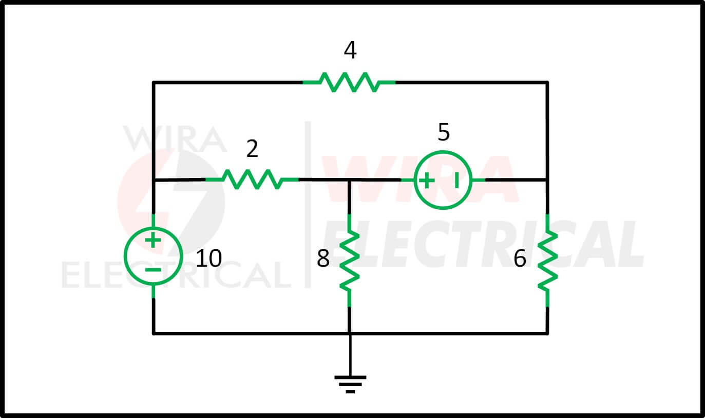
Let’s observe the simple DC circuit below and spot the difference with the previous circuit we have in nodal analysis.

Have you spotted the difference?

The circuit above only has voltage sources without a single current source. What can we get from the circuit? What is a supernode in circuit?

The circuit above has two cases:

CASE 1 – Observe the 10V source on the most left branch connected to the non reference node $v_1$ and the reference node (ground node).

This case is really simple, we don’t need to do any modification or advanced analysis. Since there is only a voltage source connected between these two nodes, the nodal voltage v1 has the same value as the voltage source.

\begin{align*}
v_{1}=10V
\end{align*}

A single voltage source in a branch really makes it simple by this knowledge of voltage.

The second case will need extra effort to solve because there is a voltage source between two nonreference nodes v2 and v3. These two nodes will form what we called generalized nodes or supernodes. We can still use KCL and KVL to calculate node voltages.

To define supernode, keep in mind that:

A supernode is formed when a voltage source is connected between two nonreference nodes and any elements connected in parallel with it.

Like we learned about nodal analysis, we only need to use KCL to find the current flowing in each branch or element.

But for a supernode, it is impossible to calculate how much current is flowing through a voltage source. What can we do then? We can use any method to calculate this but make sure to satisfy the KCL on the supernode just like any other node.

First we write the KCL equation for the circuit above,

\begin{align*}
i_{1}+i_{4}&=i_{2}+i_{3}\\
\frac{v_{1}-v_{2}}{2}+\frac{v_{1}-v_{3}}{4}&=\frac{v_{2}-0}{8}+\frac{v_{3}-0}{6}
\end{align*}

Then we use the KVL for the supernode. But before that, we have to redraw the circuit as shown below.

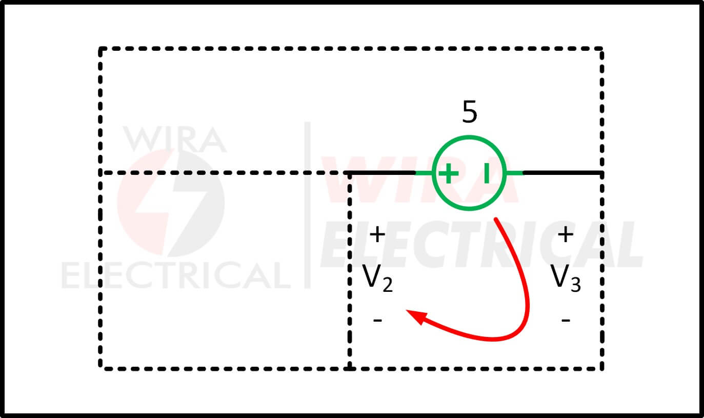
The loop in the clockwise direction gives:

\begin{align*}
-v_{2}+5+v_{3}&=0\\v_{2}-v_{3}&=5
\end{align*}

After we obtain the equations, calculating the node voltages will be easier now. After learning up to this point, we need to remember the properties of supernode analysis below:

• The voltage source inside the supernode provides the missing equation to solve all the node voltages.
• A supernode has no voltage of its own.
• A supernode requires the application of both KCL and KVL.

The Two Equations You Always Need

Every supernode problem runs on two equations working together. Get comfortable with both, because missing either one is the most common reason a solution falls apart.

KCL at the Supernode Boundary

Sum the currents crossing the boundary from outside, set the total to zero. Each resistor connected to a supernode node contributes a term:

\begin{align*}
\frac{V_{node} – V_{adjacent}}{R}
\end{align*}

where $V_{node}$​ is one of the two supernode voltages and $V_{adjacent}$​ is whatever node (or ground) sits on the other side of that resistor.

External current sources either add or subtract from the sum depending on direction. The voltage source inside? Not in the equation. Doesn’t exist as far as the boundary is concerned.

KVL Constraint: The Equation Most People Forget

Here’s where a lot of solutions go wrong. After writing the KCL equation at the supernode, some people move on — and end up with two unknowns and one equation. The system is underdetermined, and it won’t solve it.

The missing equation comes from the voltage source itself. A voltage source between nodes $V_1$​ and $V_2$, with the positive terminal at $V_1$, enforces:

\begin{align*}
V_1 – V_2 = V_s
\end{align*}

That’s a KVL constraint, and it’s exact. The source guarantees that relationship regardless of what the rest of the circuit does. Write it, and now you have two equations for two unknowns.

If you have an extended supernode — say three nodes connected by two voltage sources — you get one KCL equation at the combined boundary, and one KVL constraint per voltage source. The count always works out. Every enclosed source costs you one independent KCL equation and gives you back one KVL constraint in exchange.

Step-by-Step: How to Solve a Supernode Problem

1. Assign the reference node. Ground gets 0 V. Pick the node with the most connections if you have a choice — it minimizes the number of branches you need to deal with.
2. Label remaining nodes. $V_1$​, $V_2$​, $V_3$​… however many you have.
3. Identify supernodes. Scan for voltage sources between non-reference nodes. Each one creates a supernode. Draw the boundary on paper — seriously, draw it, don’t try to hold it mentally.
4. Write KCL at each supernode boundary. Only external branches count. Watch your signs.
5. Write the KVL constraint for each enclosed voltage source. One per source. Check polarity before writing.
6. Write KCL at any standalone nodes. Nodes not part of any supernode get their own individual KCL equations as usual.
7. Solve the system. For two unknowns, substitution works fine. Three or more, use matrix form — it’s less error-prone than chain substitution over several variables.

Supernode Analysis Examples

Now we will try to understand better from the supernode problems with answers below.

1. Observe the circuit below and find the node voltages.

Answer:

Just as we read before, a supernode is formed when a voltage source is connected between two nonreference nodes and any elements connected in parallel with it. In our case, the supernode consists of 2V source, nodes 1 and 2, and the 10Ω resistor. We remove those to redraw the circuit below:

We use the KCL for the supernode above and we get

\begin{align*}
2=i_{1}+i_{2}+7
\end{align*}

Writing the KCL equation for i1 and i2 using node voltage variables gives,

\begin{align*}
2&=\frac{v_{1}-0}{2}+\frac{v_{2}-0}{4}+7\\
8&=2v_{1}+v_{2}+28\\
v_{2}&=-20-v_{1}\tag{1.1}
\end{align*}

We are still missing the relationship between v1 and v2, we will use KVL to the circuit below.

From the clockwise loop, we get

\begin{align*}
-v_{1}-2+v_{2}&=0\\
v_{2}&=v_{1}+2\tag{1.2}
\end{align*}

From Equations.(1.1) and (1.2) we get

\begin{align*}
v_{2}=v_{1}+2&=-20-2v_{1}\\
3v_{1}=-22 \quad&\rightarrow\quad v_{1}=-7.333V
\end{align*}

we get

\begin{align*}
v_{2}=v_{1}+2=-5.333V
\end{align*}

Note that the existence of a 10Ω resistor won’t do anything because it is only connected across the supernode.

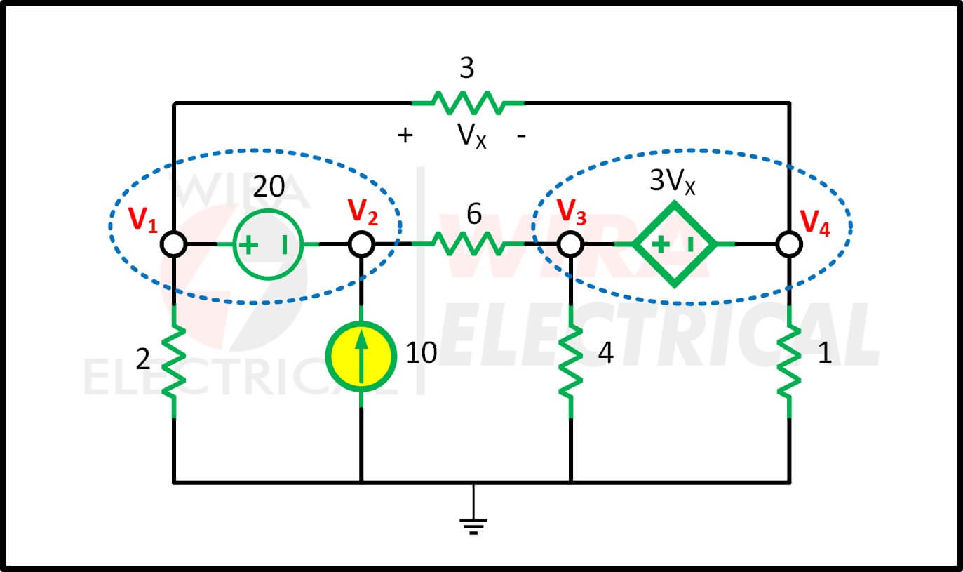
2. Find the node voltages in the circuit below. This circuit will take more time because we will do nodal analysis with 2 supernodes.

Answer:

There are two supernodes in the circuit, they are nodes 1 and 2, also nodes 3 and 4. Observe the circuit above and use KCL to two supernodes.

For supernode 1 and 2,

\begin{align*}
i_{3}+10=i_{1}+i_{2}
\end{align*}

Using the terms of the node voltages for supernode 1-2 equation gives,

\begin{align*}
\frac{v_{3}-v_{2}}{6}+10=\frac{v_{1}-v_{4}}{3}+\frac{v_{1}}{2}\\
5v_{1}+v_{2}-v_{3}-2v_{4}=60\tag{2.1}
\end{align*}

For supernode 3-4 we have the KCL equation along with its node voltages,

\begin{align*}
i_{1}&=i_{3}+i_{4}+i_{5}\\
\frac{v_{1}-v_{4}}{3}&=\frac{v_{3}-v_{2}}{6}+\frac{v_{4}}{1}+\frac{v_{3}}{4}\\
4v_{1}+2v_{2}&-5v_{3}-16v_{4}=0\tag{2.2}
\end{align*}

Next we use KVL to the branches that have voltage sources just as shown below.

For loop 1,

\begin{align*}
-v_{1}+20+v_{2}&=0\\
v_{1}-v_{2}&=20\tag{2.3}
\end{align*}

For loop 2,

\begin{align*}
-v_{3}+3v_{x}+v_{4}=0
\end{align*}

Don’t forget that

\begin{align*}
v_{x}=v_{1}-v_{4}
\end{align*}

then

\begin{align*}\tag{2.4}
3v_{1}-v_{3}-2v_{4}=0
\end{align*}

For loop 3,

\begin{align*}
v_{x}-3v_{x}+6i_{3}-20=0
\end{align*}

We know that

\begin{align*}
6i_{3}&=v_{3}-v_{2}\\
v_{x}&=v_{1}-v_{4}
\end{align*}

Hence,

\begin{align*}\tag{2.5}
-2v_{1}-v_{2}+v_{3}+2v_{4}=20
\end{align*}

In order to finish all the equations we have, we need the result of four node voltages ($v_1$​, $v_2$, $v_3$, and $v_4$). All the Equations.(2.1) to (2.5) we got earlier, we need only four to solve the remaining equations. The fifth equation is just an extra, it can be used to double-check our calculation.

Substituting Equation.(2.3) into both (2.1) and (2.2) respectively produces

\begin{align*}\tag{2.6}
6v_{1}-v_{3}-2v_{4}=80
\end{align*}

And

\begin{align*}\tag{2.7}
6v_{1}-5v_{3}-16v_{4}=40
\end{align*}

Equations.(2.4), (2.6), and (2.7) can be solved using matrix form as shown below

\begin{align*}
\begin{bmatrix}
3 & -1 & -2 \\
6 & -1 & -2 \\
6 & -5 & -16
\end{bmatrix}
\begin{bmatrix}
v_{1}\\
v_{3}\\
v_{4}
\end{bmatrix}
=
\begin{bmatrix}
0\\80\\40
\end{bmatrix}
\end{align*}

Then we use the Cramer’s rule and get

\begin{align*}
\Delta&=
\begin{vmatrix}
3 & -1 & -2 \\
6 & -1 & -2 \\
6 & -5 & -16
\end{vmatrix}=-18\\\\\
\Delta_{1}&=
\begin{vmatrix}
0 & -1 & -2 \\
80 & -1 & -2 \\
40 & -5 & -16
\end{vmatrix}
=
-480\\\\\
\Delta_{3}&=
\begin{vmatrix}3 & 0 & -2 \\
6 & 80 & -2 \\
6 & 40 & -16
\end{vmatrix}=-3120\\\\\
\Delta_{4}&=
\begin{vmatrix}
3 & -1 & 0 \\
6 & -1 & 80 \\
6 & -5 & 40
\end{vmatrix}
=
840
\end{align*}

Hence, the node voltages are

\begin{align*}
v_{1}=\frac{\Delta_{1}}{\Delta}=\frac{-480}{-18}=26.67V\\
v_{3}=\frac{\Delta_{3}}{\Delta}=\frac{-3120}{-18}=173.33V\\
v_{4}=\frac{\Delta_{4}}{\Delta}=\frac{840}{-18}=-46.67V
\end{align*}

and

\begin{align*}
v_{2}=v_{1}-20=6.667V
\end{align*}

Advantages and Limitations

Supernode analysis handles floating voltage sources cleanly and reduces the number of unknowns compared to MNA (since you don’t introduce extra current variables). For hand analysis, it’s usually the right call when the circuit has more nodes than loops and when voltage sources sit between non-reference nodes.

It’s less convenient when branch currents are the primary thing you need — you’ll have to do a second round of calculation after finding node voltages. It also gets algebraically heavy with dependent voltage sources, because the constraint equation becomes a function of circuit variables rather than a fixed number. Workable, but messier.

For large networks it’s impractical by hand regardless of method — at that scale, you’d run a simulator and not think twice about it.

Mistakes Worth Knowing About Before You Make Them

Applying KCL to just one node of the supernode. It seems like the natural thing to do. It’s wrong. The voltage source current is unknown and it shows up the moment you try. Use the boundary.

Skipping the KVL constraint. Mentioned this already, but it deserves repeating because it’s so common. If you have a supernode and you only write one equation, you’re missing the constraint. Two nodes, two equations — one from KCL, one from KVL.

Getting the polarity backwards on the constraint. If the positive terminal of the source is at $V_2$​, the constraint is $V_2 – V_1 = V_s$​, not $V_1 – V_2 = V_s$​. These are different equations and they produce different answers. Trace the polarity explicitly. Don’t guess.

Treating a source to ground as a supernode. If one terminal is grounded, that node voltage is just fixed. No supernode, no mystery. Move on.

With dependent sources, leaving the controlling variable unsubstituted. If the source value is $2V_x$​ and $V_x$​​ is a voltage across a resistor somewhere, you need to express $V_x$​​ in terms of your node voltages before the system is solvable. If you leave it as $V_x$​​, you’ve got an extra unknown with no equation for it.

Closing Thoughts

Supernode analysis is what happens when you stop trying to force a problem into a framework that doesn’t quite fit and instead step back and reframe the boundary. The voltage source isn’t a problem — it’s actually giving you information. It’s telling you exactly what the voltage difference between two nodes must be. That’s a free equation if you use it right.

The method isn’t complicated. What makes it feel complicated is the jump from writing KCL at individual nodes (which is mechanical and repetitive) to writing KCL at a compound boundary (which requires actually thinking about what’s inside and outside). Once you make that jump a few times, it becomes instinctive.

Work through three or four examples — especially ones with dependent sources or multiple supernodes — and you’ll find that the problems which initially looked like exceptions to nodal analysis are actually just a natural extension of it.

FAQ

1. Alexander, C. K., & Sadiku, M. N. O. (2021). Fundamentals of Electric Circuits (7th ed.). McGraw-Hill Education.
2. Hayt, W. H., Kemmerly, J. E., & Durbin, S. M. (2018). Engineering Circuit Analysis (9th ed.). McGraw-Hill Education.
3. Nilsson, J. W., & Riedel, S. A. (2019). Electric Circuits (11th ed.). Pearson.
4. Vlach, J., & Singhal, K. (1994). Computer Methods for Circuit Analysis and Design (2nd ed.). Springer.
5. IEEE Std 1459-2010 — IEEE Standard Definitions for the Measurement of Electric Power Quantities Under Sinusoidal, Nonsinusoidal, Balanced, or Unbalanced Conditions.