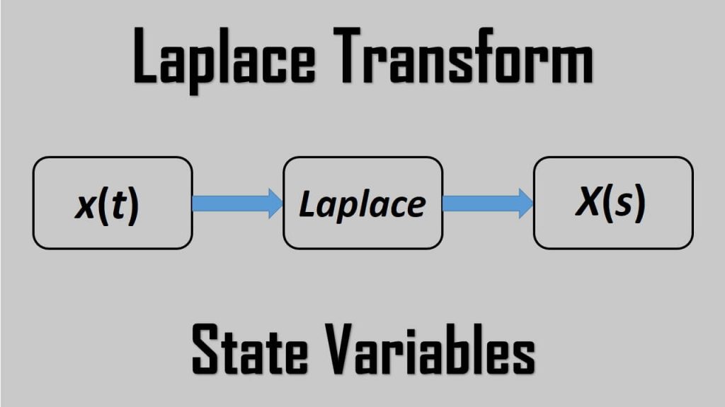
Laplace Transform State Variables Circuit Analysis
Laplace transform state variables are very useful when we are analyzing a circuit with multiple inputs and outputs.
Thus far we have considered techniques for analyzing systems with only one input and only one output.
Laplace Transform State Variables
Many engineering systems have many inputs and many outputs, as shown in Figure.(1).

The state variable method is a very important tool in analyzing systems and understanding such highly complex systems. Thus, the state variable model is more general than the single-input, single-output model, such as a transfer function.
Although the topic cannot be adequately covered in one post, we will cover it briefly at this point.
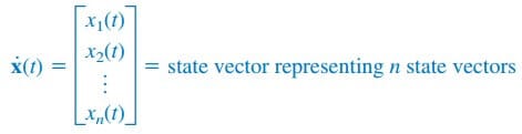
In the state variable model, we specify a collection of variables that describe the internal behaviour of the system. These variables are known as the state variables of the system.
They are the variables that determine the future behaviour of a system when the present state of the system and the input signals are known.
In other words, they are those variables which, if known, allow all other system parameters to be determined by using only algebraic equations.
A state variable is a physical property that characterizes the state of a system, regardless of how the system got to that state.
Common examples of state variables are pressure, volume, and temperature. In an electric circuit, the state variables are the inductor current and capacitor voltage since they collectively describe the energy state of the system.
The standard way to represent the state equations is to arrange them as a set of first-order differential equations:

where
and the dot represents the first derivative with respect to time, i.e.,
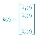
and
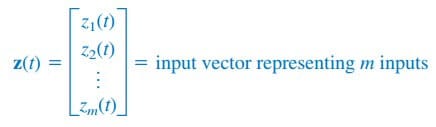
A and B are respectively n × n and n × m matrices. In addition to the state equation in Equation.(1), we need the output equation. The complete state model or state space is


where
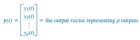
and C and D are, respectively, p × n and p × m matrices. For the special case of single-input single-output, n = m = p = 1.
Assuming zero initial conditions, the transfer function of the system is found by taking the Laplace transform of Equation.(2a); we obtain
![]()
or

where I is the identity matrix. Taking the Laplace transform of Equation.(2b) yields

Substituting Equation.(3) into (4) and dividing by Z(s) gives the transfer function as

where:
A = system matrix
B = input coupling matrix
C = output matrix
D = feedforward matrix
In most cases, D = 0, so the degree of the numerator of H(s) in Equation.(5) is less than that of the denominator. Thus,

Because of the matrix computation involved, MATLAB can be used to find the transfer function.
To apply state variable analysis to a circuit, we follow the following three steps.
Steps to Apply the State Variable Method to Circuit Analysis:
1. Select the inductor current i and capacitor voltage v as the state variables, making sure they are consistent with the passive sign convention.
2. Apply KCL and KVL to the circuit and obtain circuit variables
(voltages and currents) in terms of the state variables. This should lead to a set of first-order differential equations necessary and sufficient to determine all state variables.
3. Obtain the output equation and put the final result in state-space representation.
Steps 1 and 3 are usually straightforward; the major task is in step 2. We will illustrate this with examples.
Read also : types of diodes
Laplace Transform State Variables Examples
1. Find the state-space representation of the circuit in Figure.(2). Determine the transfer function of the circuit when vs is the input and ix is the output.
Take R = 1 Ω, C = 0.25 F, and L = 0.5 H.

Solution:
We select the inductor current i and capacitor voltage v as the state variables.


Applying KCL at node 1 gives

since the same voltage v is across both R and C. Applying KVL around the outer loop yields

Equations.(1.3) and (1.4) constitute the state equations. If we regard ix as the output,

Putting Equations.(1.3), (1.4), and (1.5) in the standard form leads to
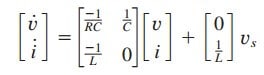

If R = 1, C = ¼, and L = ½, we obtain from Equation.(1.6) matrices

Taking the inverse of this gives
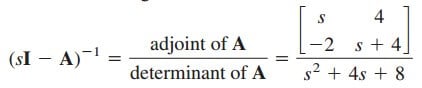
Thus, the transfer function is given by
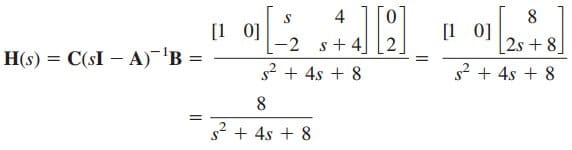
which is the same thing we would get by directly Laplace transforming the circuit and obtaining H(s) = Ix(s)∕Vs(s). The real advantage of the state variable approach comes with multiple inputs and multiple outputs.
In this case, we have one input vs and one output ix. In the next example, we will have two inputs and two outputs.
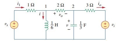
2. Consider the circuit in Figure.(3), which may be regarded as a two-input, two-output system. Determine the state variable model and fid the transfer function of the system.
Solution:
In this case, we have two inputs vs and vi and two outputs vo and io. Again, we select the inductor current i and capacitor voltage v as the state variables. Applying KVL around the left-hand loop gives

We need to eliminate i1. Applying KVL around the loop containing vs, 1-Ω resistor, 2-Ω resistor, and 1/3-F capacitor yields

But at node 1, KCL gives

Substituting this in Equation.(2.2),

Substituting this in Equation.(2.1) gives

which is one state equation. To obtain the second one, we apply KCL at
node 2.

We need to eliminate vo and io. From the right-hand loop, it is evident that

Substituting Equation.(2.4) into (2.3) gives

Substituting Equations.(2.7) and (2.8) into Equation.(2.6) yields the second state equation as

The two output equations are already obtained in Equations.(2.7) and (2.8). Putting Equations.(2.5) and (2.7) to (2.9) together in the standard form leads to the state model for the circuit, namely,


3. Assume we have a system where the output is y(t) and the input is z(t). Let the following differential equation describe the relationship between the input and the output.

Obtain the state model and the transfer function of the system.
Solution:
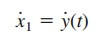
First, we select the state variables. Let x1 = y(t), therefore
Now let

Note that at this time we are looking at a second-order system that would normally have two first-order terms in the solution.
Now we have x2 = y(t), where we can find the value x2 from Equation.(3.1), i.e.,

From Equations.(3.2) to (3.4), we can now write the following matrix equations:


We now obtain the transfer function.
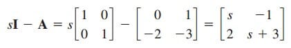 The inverse is
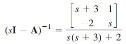 The transfer function is

To check this, we directly apply the Laplace transfer to each term in Equation.(3.1). Given that initial conditions are zero, we get
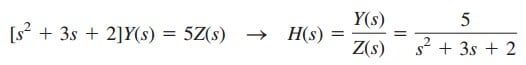
which is in agreement with what we got previously.