Inverse Laplace Transform Formula and Simple Examples
Inverse Laplace transform is used when we want to convert the known Laplace equation into the time-domain equation.
Even if we have the table conversion from Laplace transform properties, we still need to so some equation simplification to match with the table.
The Inverse Laplace Transform
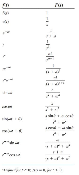
Given F (s), how do we transform it back to the time domain and obtain the corresponding f (t)? By matching entries in Table.(2) in the ‘Laplace Transform Properties‘ (let’s put that table in this post as Table.1 to ease our study)
we avoid using Equation.(5) in ‘Laplace Transform Definition’ to find f (t).
Suppose F (s) has the general form of

where N(s) is the numerator polynomial and D(s) is the denominator polynomial. The roots of N(s) = 0 are called the zeros of F (s), while
the roots of D(s) = 0 are the poles of F (s). Although Equation.(1) is similar in form to Equation.(3) in ‘Transfer Function’, here F (s) is the Laplace transform of a function, which is not necessarily a transfer function.
We use partial fraction expansion to break F (s) down into simple terms whose inverse transform we obtain from Table.(1).
Thus, finding the inverse Laplace transform of F (s) involves two steps.
Steps to Find the Inverse Laplace Transform :
Decompose F (s) into simple terms using partial fraction expansion.
Find the inverse of each term by matching entries in Table.(1).
Let us consider the three possible forms F (s ) may take and how to apply the two steps to each form.
Laplace Transform Simple Poles
A simple pole is the first-order pole. If F ( s ) has only simple poles, then D (s ) becomes a product of factors, so that

where s = −p1, −p2,…, −pn are the simple poles, and pi ≠ pj for all i ≠ j (i.e., the poles are distinct). Assuming that the degree of N(s) is less than the degree of D(s), we use partial fraction expansion to decompose F(s) in Equation.(2) as

The expansion coefficients k1, k2,…,kn are known as the residues of F(s). There are many ways of finding the expansion coefficients.
One way is using the residue method. If we multiply both sides of the Equation.(3) by (s + p1), we obtain

Since pi ≠ pj, setting s = −p1 in Equation.(4) leaves only k1 on the right-hand side of Equation.(4). Hence,

Thus, in general,

This is known as Heaviside’s theorem. Once the values of ki are known, we proceed to find the inverse of F(s) using Equation.(3).
Since the inverse transform of each term in Equation.(3) is
L−1 [k/(s + a)] = ke−atu(t),
then, from Table 15.1 in the ‘Laplace Transform Properties’,

Laplace Transform Repeated Poles
Suppose F(s) has n repeated poles at s = −p. Then we may represent
F(s) as

where F1(s) is the remaining part of F(s) that does not have a pole at s = −p. We determine the expansion coefficient kn as

as we did above. To determine kn −1, we multiply each term in Equation.(8) by (s + p)n and differentiate to get rid of kn, then evaluate the result at s = −p to get rid of the other coefficients except kn−1. Thus, we obtain

Repeating this gives

The mth term becomes

where m = 1, 2,…,n − 1. One can expect the differentiation to be difficult to handle as m increases. Once we obtain the values of k1, k2,…,kn by partial fraction expansion, we apply the inverse transform

to each term in the right-hand side of Equation.(8) and obtain

Read also : laplace transform circuit
Laplace Transform Complex Poles
A pair of complex poles is simple if it is not repeated; it is a double or multiple poles if repeated. Simple complex poles may be handled the same as simple real poles, but because complex algebra is involved the result is always cumbersome.
An easier approach is a method known as completing the square. The idea is to express each complex pole pair (or quadratic term) in D(s) as a complete square such as
(s + α)2 + β2
and then use Table.(1) to find the inverse of the term.
Since N(s) and D(s) always have real coefficients and we know that the complex roots of polynomials with real coefficients must occur in conjugate pairs, F(s) may have the general form

where F1(s) is the remaining part of F(s) that does not have this pair of complex poles. If we complete the square by letting

and we also let
then Equation.(15) becomes

From Table.(1), the inverse transform is
The sine and cosine terms can be combined. Whether the pole is simple, repeated, or complex, a general approach that can always be used in finding the expansion coefficients is the method of algebra.
To apply the method, we first set F(s) = N(s)/D(s) equal to an expansion containing unknown constants. We multiply the result through by a common denominator. Then we determine the unknown constants by equating coefficients (i.e., by algebraically solving a set of simultaneous equations for these coefficients at like powers of s).
Another general approach is to substitute specific, convenient values of s to obtain as many simultaneous equations as the number of unknown coefficients, and then solve for the unknown coefficients. We must make sure that each selected value of s is not one of the poles of F(s). The example below illustrates this idea.
Inverse Laplace Transform Examples
Let us review the laplace transform examples below:
Inverse Laplace Transform Example 1
Find the inverse Laplace transform of

Solution:
The inverse transform is given by

where Table.(1) has been consulted for the inverse of each term.
Inverse Laplace Transform Example 2
Find f (t) given that

Solution:
Unlike in the previous example where the partial fractions have been provided, we first need to determine the partial fractions. Since there are three poles, we let

where A, B, and C are the constants to be determined. We can find the constants using two approaches.
METHOD 1 : Residue method

METHOD 2 : Algebraic method
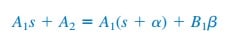
Multiplying both sides of Equation.(2.1) by s(s + 2)(s + 3) gives
![]()
or
![]()
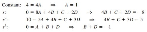
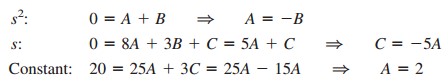
Equating the coefficients of like powers of s gives

Thus A = 2, B = −8, C = 7, and Equation.(2.1) becomes
 By finding the inverse transform of each term, we obtain
![]()
Inverse Laplace Transform Example 3
Calculate v (t ) given that
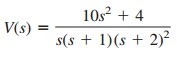 Solution:
While the previous example is on simple roots, this example is on repeated roots. Let

METHOD 1 : Residue method

METHOD 2 : Algebraic method

Equating coefficients,
Solving these simultaneous equations gives A = 1, B = −14, C = 22, D = 13, so that

Taking the inverse transform of each term, we get
![]()
Inverse Laplace Transform Example 4
Find the inverse transform of the frequency-domain function in
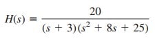
Solution:
In this example, H(s) has a pair of complex poles at s2 + 8s + 25 = 0 or s = −4 ± j3. We let
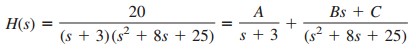
We now determine the expansion coefficients in two ways.
METHOD 1 : Combination of methods.
We can obtain A using the method of residue,
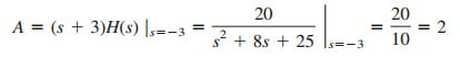
Although B and C can be obtained using the method of residue, we will not do so, to avoid complex algebra. Rather, we can substitute two specific values of s [say s = 0, 1, which are not poles of F (s)] into Equation.(4.1).
This will give us two simultaneous equations from which to find B and C. If we let s = 0 in Equation.(4.1), we obtain
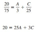
Since A = 2, Equation.(4.2) gives C = −10. Substituting s = 1 into Equation.(4.2) gives

But A = 2, C = −10, so that Equation.(4.3) gives B = −2.
METHOD 2 : Algebraic method.
Multiplying both sides of Equation.(4.1) by (s + 3)(s2 + 8s + 25) yields

Equating coefficients,
That is, B = −2, C = −10. Thus

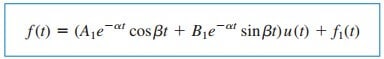
Taking the inverse of each term, we obtain

It is alright to leave the result this way. However, we can combine the cosine and sine terms as

Next, we determine the coefficient A and the phase angle θ:
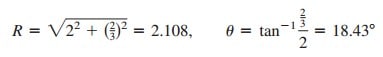
Thus,
![]()