Complete Explanation and Example Laplace Transform Properties
The Laplace transform properties provide us with easy mathematical transformation quickly.
The properties of the Laplace transform help us to obtain transform pairs without directly using the equations in previous post about the definition of Laplace transform. As we derive each of these properties, we should keep in mind the definition of the Laplace transform.
Laplace Transform Properties
Laplace Transform Linearity
If F1(s) and F2(s) are, respectively, the Laplace transforms of f1(t) and f2(t), then
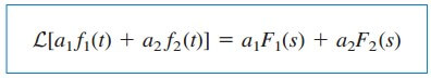
where a1 and a2 are constants. Equation.(1) expresses the linearity property of the Laplace transform. The proof of Equation.(1) follows readily from the definition of the Laplace transform in the Equation.(1) in Laplace Transform Definition.
For example, by the linearity property in Equation.(1), we may write

But from the Laplace Transform Definition Example 2, L[e–at] = 1/(s + a). Hence,

Laplace Transform Scaling
If F(s) is the Laplace transform of f(t), then

where a is a constant and a > 0. If we let x = at, dx = a dt, then

Comparing this integral with the Equation.(1) in Laplace Transform Definition shows that s in that equation must be replaced by s/a while the dummy variable t is replaced by x. Hence, we obtain the scaling property as

For example, we know from the Laplace Transform Definition Example 2 that

Using the scaling property in Equation.(6),

which may also be obtained from Equation.(7) by replacing ω with 2ω.
Laplace Transform Time Shift
If F(s) is the Laplace transform of f(t), then

But u(t − a) = 0 for t < a and u(t − a) = 1 for t > a. Hence,

If we let x = t – a, then dx = dt and t = x + a. As t → a, x → 0 and
as t → ∞, x → ∞. Thus,
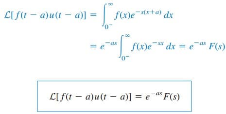
In other words, if a function is delayed in time by a, the result in the s domain is multiplying the Laplace transform of the function (without the delay) by e–as. This is called the time-delay or time-shift property of the Laplace transform.
As an example, the Equation.(3) using time-shift property in Equation.(11) will result

Laplace Transform Frequency Shift
If F(s) is the Laplace transform of f(t), then

That is, the Laplace transform of e–atf(t) can be obtained from the Laplace transform of f(t) by replacing every s with s + a. This is known as frequency shift or frequency translation.
As an example, we know that

Using the shift property in Equation.(13), we obtain the Laplace transform of the damped sine and damped cosine functions as


Laplace Transform Time Differentiation
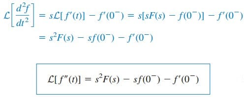
Given that F(s) is the Laplace transform of f(t), the Laplace transform of its derivative is

To integrate this by parts, we let u = e–st, du = –se–st dt, and dv = (df/dt) dt = df(t), v = f(t). Then

The Laplace transform of the second derivative of f (t) is a repeated application of Equation.(17) as
Continuing in this manner, we can obtain the Laplace transform of the nth derivative of f(t) as

As an example, we can use Equation.(17) to obtain the Laplace transform of the sine from that of the cosine. If we let f(t) = cos ωt, then f(0) = 1 and f(t) = –ω sin ωt. Using Equation.(17) and the scaling property,

as expected.
Laplace Transform Time Integration
If F(s) is the Laplace transform of f(t), the Laplace transform of its integral is

To integrate this by parts, we let
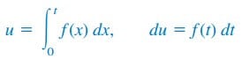
and
Then
 For the first term on the right-hand side of the equation, evaluating the term at t = ∞ yields zero due to e–s∞ and evaluating it at t = 0 gives
Thus, the first term is zero, and
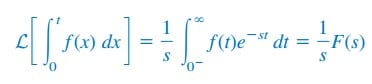 or simply

As an example, if we let f(t) = u(t), F(s) = 1/s. Using Equation.(22),

Thus, the Laplace transform of the ramp function is

Applying Eq. (15.28), this gives

Repeated applications of Equation.(22) lead to

Similarly, using integration by parts, we can show that

where
Laplace Transform Frequency Differentiation
If F(s) is the Laplace transform of f(t), then
Taking the derivative with respect to s,
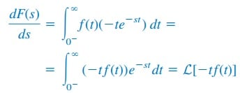
and the frequency differentiation property becomes

Repeated applications of this equation lead to

For example, we know that L[e–at] = 1/(s + a). Using the property in Equation.(27),

Note that if a = 0, we obtain L[t] = 1/s2 as in Equation.(23), and repeated applications of Equation.(27) will yield Equation.(25).
Laplace Transform Time Periodicity
If function f(t) is a periodic function such as shown in Figure.(1)

it can be represented as the sum of time-shifted functions shown in Figure.(2).

Thus,

where f1(t) is the same as the function f(t) gated over the interval 0 < t < T, that is,

or

We now transform each term in Equation.(30) and apply the time-shift property in Equation.(11). We obtain

But

if |x| < 1. Hence,

where F1(s) is the Laplace transform of f1(t); in other words, F1(s) is the transform f(t) defined over its first period only. Equation.(34) shows that the Laplace transform of a periodic function is the transform of the first period of the function divided by 1 − e−T s.
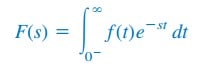
Laplace Transform Initial and Final Values
The initial-value and final-value properties allow us to find the initial value f (0) and the final value f (∞) of f (t) directly from its Laplace transform F (s). To obtain these properties, we begin with the differentiation property in Equation.(17), namely,

If we let s → ∞, the integrand in Equation.(35) vanishes due to the damping exponential factor, and Equation.(35) becomes

This is known as the initial-value theorem. For example, we know from Equation.(15a) that

Using the initial-value theorem,
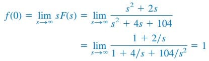
which confirms what we would expect from the given f (t).
In Equation.(35), we let s → 0; then
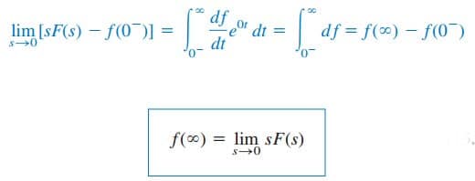
This is referred to as the final-value theorem. In order for the final-value theorem to hold, all poles of F (s) must be located in the left half of the s plane; that is, the poles must have negative real parts.
The only exception to this requirement is the case in which F (s) has a simple pole at s = 0, because the effect of 1/s will be nullified by sF (s) in Equation.(38). For example, from Equation.(15b),

Applying the final-value theorem,
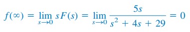
as expected from the given f (t). As another example,

so that
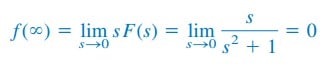 This is incorrect, because f (t) = sin t oscillates between +1 and −1 and does not have a limit as t → ∞.
Thus, the final-value theorem cannot be used to find the final value of f (t) = sin t, because F (s) has poles at s = ±j, which are not in the left half of the s plane.
In general, the final-value theorem does not apply in finding the final values of sinusoidal functions—these functions oscillate forever and do not have final values.
The initial-value and final-value theorems depict the relationship between the origin and infinity in the time domain and the s domain. They serve as useful checks on Laplace transforms.
Table.(1) provides a list of the properties of the Laplace transform. There are other properties, but these are enough for present purposes.
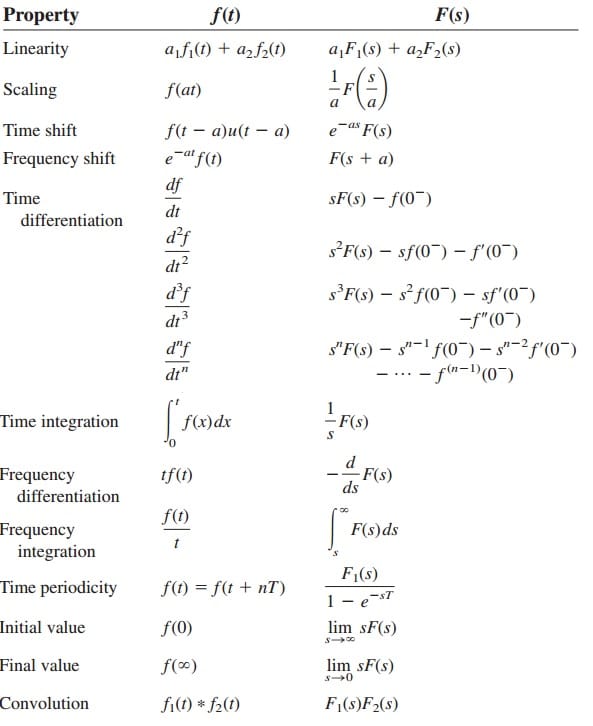
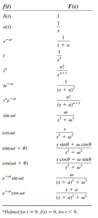
Table.(2) summarizes the Laplace transforms of some common functions. We have omitted the factor u(t) except where it is necessary.
Read also : linear transformers
Laplace Transform Properties Examples
Let’s review the Laplace transform properties below:
Laplace Transform Properties Example 1
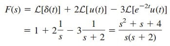
Obtain the Laplace transform of f(t) = δ(t) + 2u(t) − 3e−2t, t ≥ 0.
Solution:
By the linearity property,
Laplace Transform Properties Example 2
Determine the Laplace transform of f (t) = t2 sin 2t u(t).
Solution:
We know that
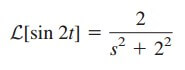
Using frequency differentiation in Equation.(28),
Laplace Transform Properties Example 3
Find the Laplace transform of the gate function in Figure.(3).

Solution:
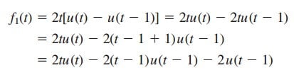
We can express the gate function in Figure.(3) as
![]()
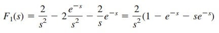
Since we know the Laplace transform of u(t), we apply the time-shift property and obtain
Laplace Transform Properties Example 4
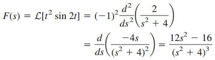
Calculate the Laplace transform of the periodic function in Figure.(4).

Solution:
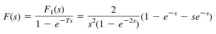
The period of the function is T = 2. To apply Equation.(34), we first obtain the transform of the first period of the function.
Using the time-shift property,
Thus, the transform of the periodic function in Figure.(4) is
Laplace Transform Properties Example 5
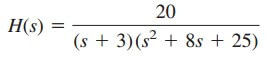
Find the initial and final values of the function whose Laplace transform
is
Solution:
Applying the initial-value theorem,

To be sure that the final-value theorem is applicable, we check where the poles of H(s) are located. The poles of H(s) are s = −3, −4 ± j3, which all have negative real parts: they are all located on the left half of
the s plane in Figure.(5). Hence the final-value theorem applies and
Both the initial and final values could be determined from h(t) if we knew it.