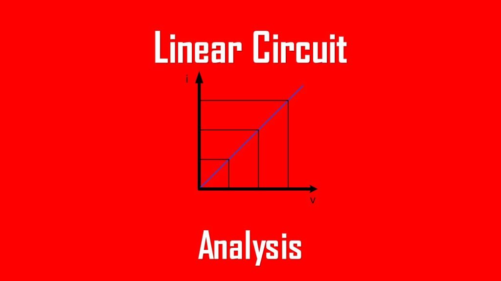
Linear Circuit Analysis vs Nonlinear Circuits
Linear circuit analysis will help us greatly when we are attempting to analyze a more complex circuit like what we haven’t encountered before.
Linear Circuit Analysis
A linear circuit is a circuit that consists only of linear elements. Its output is linearly proportional to its input, increased or decreased by a constant.
Since we have learned about Kirchhoff’s laws, we may think we have everything we need to solve every kind of electrical circuit.
Analyzing circuits with Kirchhoff’s laws comes with major advantages and disadvantages.
The major advantage is we don’t need to tamper the circuit’s original configuration.
The major disadvantage is we need extra computation for larger, more complex circuits.
The more technology advances, the more methods we need to use to make sure our analysis is properly done, and of course with the least simplicity.
From this need, more linearity theorems were invented including:
These two are applicable to a linear circuit, but first we need to understand what a linear circuit is.
What is a Linear Circuit
Just from its name implies, a linear circuit is a circuit where linearity is fulfilled. Linearity is a property of an element which describes the linear relationship between cause and effect, start and end, any two variables with a common thing such as electrical current and voltage.
Linearity property is the combination of homogeneity (scaling) property and additivity property.
In a linear circuit we will learn about homogeneity properties.
Law of homogeneous circuits states that if an input (or excitation) is multiplied by a constant, the output (or response) is also multiplied by the same constant.
We will use a resistor this time to simplify our study.
Observe the simple Ohm’s law equation below:
![]()
If the current (i) is increased then the voltage (v) is also increased. Let’s say the current is amplified by a constant k, then the voltage is also increased by the constant k.
Or we can spill it to make it easier to understand, homogeneity can be understood from the equation below.
![]()
We have learned about homogeneity, it is time for additive property.
The additivity property requires that the response to a sum of inputs is the sum of the responses to each input applied separately. Using the voltage-current relationship of a resistor, if
![]()
And
![]()
Applying (i1 + i2) results

From all of the explanations above, we can be sure that a resistor is a linear element because the voltage-current relationship fulfills the requirement of homogeneity property and additivity property.
In conclusion,
A linear circuit is when its output is linearly related or proportional to its input.
So what is a simple example of a nonlinear circuit?
One of the simple example of a nonlinear property is the equation for calculating power
![]()
This equation forms a quadratic function, thus the relationship between voltage and power or current and power is nonlinear.
Therefore, the theorems mentioned in this post will not be applicable to power calculation.
Linearity Theorem
To understand further about linearity property, let us read the principle behind the linearity theorems (those will be covered in other posts).
Observe the circuit below, a linear circuit supplied by an independent voltage source (vs), loaded with a resistor (R), and no independent sources inside it.

The electric current (i) is flowing through the load R.
Assume that the voltage source, vs = 10V with the resistance, R = 5Ω.
The current will be 2 A.
Assume that the voltage source, vs = 1V with the resistance, R = 5Ω.
The current will be 0.2 A.
This proves the linearity property for the voltage-current relationship with a fully resistive load.
A linear circuit diagram will form a perfect triangle between two parameters, as an example, a resistive circuit and its voltage-current relationship diagram as shown below.

Linear Circuit Example
Let us solve a few simple circuits below for our practice.
1. Observe the circuit below, and find the value of Io, if vx = 12 V and vs = 24 V.

Using KVL to both loops, we get
![]()
For the left loop, and
![]()
For the right loop.
Since vx = 2i1, then Equation(1.2) becomes
![]()
Summing Equations(1.1) and (1.3) results
![]()
Substituting this with Equation(1.1) we get
![]()
If vs = 12 V, then
![]()
If vs = 24 V, then
![]()
Conclude that if we double the voltage, the current will be doubled.
Thus this circuit is a linear circuit.
2. Observe the circuit below and find the actual value of Io.

Assume that Io = 1 A first to make it very simple to solve.
Then,
![]()
And
![]()
Then using KCL at node 1 results

Using KCL at node 2 results
![]()
Hence,
![]()
Thus, with the assumed value of Io = 1 A (Io1) will generate Is = 5 A (Is1)
If we have the actual value of Is = 15 A (Is2) then the actual value of Io (Io2) will be

The actual value of Io in our circuit is 3 A.
Linear and Nonlinear Circuits
We have learned about a linear circuit, so what is the difference with a nonlinear circuit?
A linear circuit consists only of linear elements while a nonlinear circuit consists of at least one nonlinear element.
Just as stated above,
A linear circuit is a circuit that consists only of linear elements. Its output is linearly proportional to its input, increased or decreased by a constant.
A nonlinear circuit is a circuit that consists of at least one nonlinear element. Its output is not linearly proportional to its input.
The most common nonlinear element is a diode.
Why?
If you have learned about diode, you should have known its current-voltage relationship diagram looks like

Since we can’t directly calculate the current or voltage based on a constant, this one is a nonlinear element, thus using this will make a nonlinear circuit.
To summarize the difference between a linear circuit with a nonlinear circuit, we can observe the comparisons below:
- A linear circuit only consists of linear element(s) while a nonlinear circuit consists of at least one nonlinear element.
- Superposition theorem is only applicable to linear circuits and not applicable to nonlinear circuits.
- Thevenin’s theorem is only applicable to linear circuits and not applicable to nonlinear circuits.
- Norton’s theorem is only applicable to linear circuits and not applicable to nonlinear circuits.
- The output curve in linear circuits is a perfectly straight line while a nonlinear circuit has unique output curves and commonly they are not perfectly straight lines.
- A linear circuit fulfills homogeneity and additivity properties, a nonlinear circuit does not fulfill them.
Few example of linear circuit elements are:
- Resistor
- Inductor
- Capacitor
Few example of nonlinear circuit elements are:
- Diode
- Transistor
- Transformer