Bode Plot Examples
In this post we will learn about Bode Plot Examples and the explanation behind it to help us analyze and utilize bode plot, along with how to read a bode plot.
The frequency range required in frequency response is often so wide that it is inconvenient to use a linear scale for the frequency axis. Also, there is a more systematic way of locating the important features of the magnitude and phase plots of the transfer function.
For these reasons, it has become standard practice to use a logarithmic scale for the frequency axis and a linear scale in each of the separate plots of magnitude and phase.
Transfer Function from Bode Plot Examples
Such semilogarithmic plots of the transfer function—known as Bode plots—have become the industry standard.
Bode plots are semi log plots of the magnitude (in decibels) and phase (in degrees) of a transfer function versus frequency.
Bode plots contain the same information as the non logarithmic plots discussed in the previous section, but they are much easier to construct, as we shall see shortly.
The transfer function can be written as
![]()
Taking the natural logarithm of both sides,
![]()
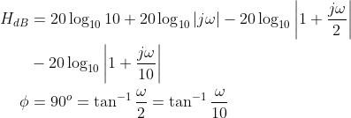
Thus, the real part of ln H is a function of the magnitude while the imaginary part is the phase. In a Bode magnitude plot, the gain
![]()
is plotted in decibels (dB) versus frequency.
In a Bode phase plot, 𝜙 is plotted in degrees versus frequency. Both magnitude and phase plots are made on semilog graph paper.
A transfer function in the form of the equation above may be written in terms of factors that have real and imaginary parts. One such representation might be
![]()
which is obtained by dividing out the poles and zeros in H(ω). The representation of H(ω) as in the equation above is called the standard form. In this particular case, H(ω) has seven different factors that can appear in various combinations in a transfer function. Transfer function from bode plot examples are:
- A gain K
- A pole (jω)−1 or zero (jω) at the origin
- A simple pole 1/(1 + jω/p1) or zero (1 + jω/z1)
- A quadratic pole 1/[1 + j2ζ2ω/ωn + (jω/ωn)2] or zero [1 + j2ζ1ω/ωk + (jω/ωk)2]
In constructing a Bode plot, we plot each factor separately and then combine them graphically. The factors can be considered one at a time and then combined additively because of the logarithms involved.
Bode Diagram Examples
It is this mathematical convenience of the logarithm that makes Bode plots a powerful engineering tool.
We will now make straight-line plots of the factors listed above. We shall find that these straight-line plots known as Bode plots approximate the actual plots to a surprising degree of accuracy.
Now we will try to understand bode plot solved examples below.
Constant term: For the gain K, the magnitude is 20 log10 K and the phase is 0o; both are constant with frequency. Thus the magnitude and phase plots of the gain are shown below. If K is negative, the magnitude remains 20 log10|K| but the phase is ±180o.

Pole/zero at the origin: For the zero (jω) at the origin, the magnitude is 20 log10 ω and the phase is 90o. These are plotted below, where we notice that the slope of the magnitude plot is 20 dB/decade, while the phase is constant with frequency.

A decade is an interval between two frequencies with a ratio of 10; e.g., between ω0 and 10ω0, or between 10 and 100 Hz. Thus, 20 dB/decade means that the magnitude changes 20 dB whenever the frequency changes tenfold or one decade.
The Bode plots for the pole (jω)−1 are similar except that the slope of the magnitude plot is −20 dB/decade while the phase is −90o. In general, for (jω)N, where N is an integer, the magnitude plot will have a slope of 20N dB/decade, while the phase is 90N degrees.
Simple pole/zero: For the simple zero (1 + jω/z1), the magnitude is 20 log10 |1 + jω/z1| and the phase is tan−1 ω/z1. We notice that
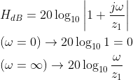
showing that we can approximate the magnitude as zero (a straight line with zero slope) for small values of ω and by a straight line with slope 20 dB/decade for large values of ω.
The frequency ω = z1 where the two asymptotic lines meet is called the corner frequency or break frequency.
Thus the approximate magnitude plot is shown below, where the actual plot is also shown.

Notice that the approximate plot is close to the actual plot except at the break frequency, where ω = z1 and the deviation is 20 log10|(1 + j1)| = 20 log10 √2 = 3 dB.
The phase tan−1(ω/z1) can be expressed as
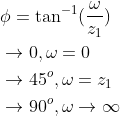
As a straight-line approximation, we let 𝜙 ≅ 0 for ω ≤ z1/10, 𝜙 ≅ 45o for ω = z1, and 𝜙 ≅ 90o for ω ≥ 10z1. As shown in the graph above along with the actual plot, the straight-line plot has a slope of 45o per decade.
The Bode plots for the pole 1/(1 + jω/p1) are similar to those above except that the corner frequency is at ω = p1, the magnitude has a slope of −20 dB/decade, and the phase has a slope of −45o per decade.
Quadratic pole/zero: The magnitude of the quadratic pole 1 /[1 + j2 ζ2 ω /ωn + (jω/ωn)2] is −20 log10 |1 + j2ζ2ω/ωn + (jω/ωn)2| and the phase is −tan−1 (2ζ2ω/ωn)/(1 − ω/ωn2). But
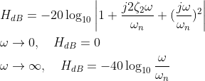
Thus, the amplitude plot consists of two straight asymptotic lines: one with zero slope for ω < ωn and the other with slope -40dB/decade for ω > ωn, with ωn as the corner frequency. The graph below shows the bode diagram example.

Note that the actual plot depends on the damping factor ζ2 as well as the corner frequency ωn.
The significant peaking in the neighborhood of the corner frequency should be added to the straight-line approximation if a high level of accuracy is desired.
However, we will use the straight-line approximation for the sake of simplicity.
The phase can be expressed as
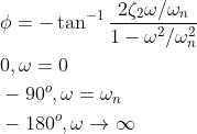
The phase plot is a straight line with a slope of 90o per decade starting at ωn/10 and ending at 10ωn, as shown above.
We see again that the difference between the actual plot and the straight-line plot is due to the damping factor.
Notice that the straight-line approximations for both magnitude and phase plots for the quadratic pole are the same as those for a double pole, i.e. (1 + jω/ωn)−2.
We should expect this because the double pole (1 + jω/ωn)−2 equals the quadratic pole 1/[1 + j2ζ2ω/ωn + (jω/ωn)2] when ζ2 = 1.
Thus, the quadratic pole can be treated as a double pole as far as straight-line approximation is concerned.
For the quadratic zero [1 +j2ζ1ω/ωk +(jω/ωk)2], the plots in the graph above are inverted because the magnitude plot has a slope of 40 dB/decade while the phase plot has a slope of 90o per decade.
To sketch the Bode plots for a function H(ω) in the form of the equation above, for example, we first record the corner frequencies on the semilog graph paper, sketch the factors one at a time as discussed above, and then combine additively the graphs of the factors.
The combined graph is often drawn from left to right, changing slopes appropriately each time a corner frequency is encountered. The following examples illustrate this procedure.
This is a bode plot explained.
Bode Plot Examples
Let’s review the bode plots examples below:
1. Construct the Bode plots for the transfer function
![]()
Answer:
We first put H(ω) in the standard form by dividing out the poles and zeros. Thus,
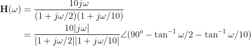
Hence the magnitude and phase are
We notice that there are two corner frequencies at ω = 2, 10. For both the magnitude and phase plots, we sketch each term as shown by the dotted lines below. We add them up graphically to obtain the overall plots shown by the solid curves.

2. Obtain the Bode plots for
![]()
Answer:
Putting H(ω) in the standard form, we get
![]()
From this, we obtain the magnitude and phase as
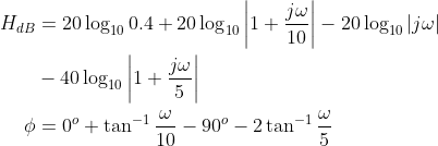
There are two corner frequencies at ω = 5, 10 rad/s. For the pole with corner frequency at ω = 5, the slope of the magnitude plot is −40 dB/decade and that of the phase plot is −90o per decade due to the power of 2.
The magnitude and the phase plots for the individual terms (in dotted lines) and the entire H(jω) (in solid lines) are below.

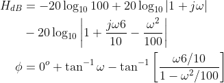
3. Draw the Bode plots for
![]()
Answer:
We express H(s) as
![]()
For the quadratic pole, ωn = 10 rad/s, which serves as the corner frequency. The magnitude and phase are
Graph below shows the Bode plots. Notice that the quadratic pole is treated as a repeated pole at ωk, that is, (1 + jω/ωk)2, which is an approximation.

4. Given the Bode plot in the graph below, obtain the transfer function H(ω).

Answer:
To obtain H(ω) from the Bode plot, we keep in mind that a zero always causes an upward turn at a corner frequency, while a pole causes a downward turn.
We notice from the graph above that there is a zero j ω at the origin which should have intersected the frequency axis at ω = 1. This is indicated by the straight line with slope +20 dB/decade.
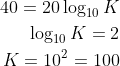
The fact that this straight line is shifted by 40 dB indicates that there is a 40-dB gain; that is,
In addition to the zero j ω at the origin, we notice that there are three factors with corner frequencies at ω = 1 , 5, and 20 rad/s. Thus, we have:
- A pole at p = 1 with slope −20 dB/decade to cause a downward turn and counteract the pole at the origin. The pole at z = 1 is determined as 1 /(1 + jω/1).
- Another pole at p = 5 with slope −20 dB/decade causing a downward turn. The pole is 1/(1 + jω/5).
- A third pole at p = 20 with slope −20 dB/decade causing a further downward turn. The pole is 1/(1 + jω/20).
Putting all these together gives the corresponding transfer function as