Laplace Transform Convolution Integral Complete Examples
The Laplace transform convolution integral is one of the applications of the Laplace transform.
The convolution of two signals consists of time-reversing one of the signals, shifting it, and multiplying it point by point with the second signal, and integrating the product.
Laplace Transform Convolution Integral
The term convolution means “folding.” A convolution is an invaluable tool for the engineer because it provides a means of viewing and characterizing physical systems.
For example, it is used in finding the response y(t) of a system to an excitation x(t), knowing the system impulse response h(t). This is achieved through the convolution integral, defined as

or simply

where λ is a dummy variable and the asterisk denotes convolution. Equations.(1) or (2) states that the output is equal to the input convolved with the unit impulse response. The convolution process is commutative:

or

This implies that the order in which the two functions are convolved is immaterial. We will see shortly how to take advantage of this commutative property when performing graphical computation of the convolution integral.
The convolution of two signals consists of time-reversing one of the signals, shifting it, and multiplying it point by point with the second signal, and integrating the product.
The convolution integral in Equation.(1) is the general one; it applies to any linear system. However, the convolution integral can be simplified if we assume that a system has two properties.
First, if
x(t) = 0 for t < 0,
then

Second, if the system’s impulse response is causal
i.e., h(t) = 0 for t < 0, then
h(t − λ) = 0 for t − λ < 0 or λ > t,
so that Equation.(4) becomes

Here are some properties of the convolution integral.
Before learning how to evaluate the convolution integral in Equation.(5), let us establish the link between the Laplace transform and the convolution integral.
Given two functions f1(t) and f2(t) with Laplace transforms F1(s) and F2(s), respectively, their convolution is

Taking the Laplace transform gives

To prove that Equation.(7) is true, we begin with the fact that F1(s) is defined as

Multiplying this with F2(s) gives

We recall from the time shift property that the term in brackets can be written as

Substituting Equation.(10) into Equation.(9) gives

Interchanging the order of integration results in

The integral in brackets extends only from 0 to t because the delayed unit step u(t − λ) = 1 for λ < t and u(t − λ) = 0 for λ > t. We notice that the integral is the convolution of f1(t) and f2(t) as in Equation.(6).
Hence,

as desired. This indicates that convolution in the time domain is equivalent to multiplication in the s domain.
For example, if
x(t) = 4e−t and h(t) = 5e−2t,
applying the property in Equation.(13), we get

Although we can find the convolution of two signals using Equation.(13), as we have just done, if the product F1(s)F2(s) is very complicated, finding the inverse may be tough.
Also, there are situations in which f1(t) and f2(t) are available in the form of experimental data and there are no explicit Laplace transforms. In these cases, one must do the convolution in the time domain.
The process of convolving two signals in the time domain is better appreciated from a graphical point of view. The graphical procedure for evaluating the convolution integral in Equation.(5) usually involves four steps.
Steps to Evaluate the Convolution Integral:
1. Folding: Take the mirror image of h(λ) about the ordinate axis to
obtain h(−λ).
2. Displacement: Shift or delay h(−λ) by t to obtain h(t − λ).
3. Multiplication: Find the product of h(t − λ) and x(λ).
4. Integration: For a given time t, calculate the area under the
product h(t − λ)x(λ) for 0 < λ < t to get y(t) at t.
The folding operation in step 1 is the reason for the term convolution. The function h(t − λ) scans or slides over x(λ). In view of this superposition procedure, the convolution integral is also known as the superposition integral.
To apply the four steps, it is necessary to be able to sketch x(λ) and h(t − λ). To get x(λ) from the original function x(t) involves merely replacing t with λ. Sketching h(t − λ) is the key to the convolution process.
It involves reflecting h(λ) about the vertical axis and shifting it by t. Analytically, we obtain h(t − λ) by replacing every t in h(t) by t − λ.
Since convolution is commutative, it may be more convenient to apply steps 1 and 2 to x(t) instead of h(t). The best way to illustrate the procedure is with some examples.
Read also : laplace transform network stability
Laplace Transform Convolution Integral Examples
Let’s review the Laplace transform convolution integral examples below:
Laplace Transform Convolution Integral Example 1
Find the convolution of the two signals in Figure.(1).

Solution:
We follow the four steps to get
y (t ) = x1(t) ∗ x2(t).
First, we fold x1(t) as shown in Figure.(2a) and shift it by t as shown in Figure.(2b). For different values of t, we now multiply the two functions and integrate to determine the area of the overlapping region.

For 0 < t < 1, there is no overlap of the two functions, as shown in Figure.(3a).

Hence,

For 1 < t < 2, the two signals overlap between 1 and t, as shown in Figure.(3b).

For 2 < t < 3, the two signals completely overlap between (t − 1) and t, as shown in Figure.(3c). It is easy to see that the area under the curve is 2. Or

For 3 < t < 4, the two signals overlap between (t − 1) and 3, as shown in Figure.(3d).

For t > 4, the two signals do not overlap [Figure.(3e)], and

Combining Equations.(1.1) to (1.5), we obtain

which is sketched in Figure.(4). Notice that y(t) in this equation is continuous. This fact can be used to check the results as we move from one range of t to another.

The result in Equation.(1.6) can be obtained without using the graphical procedure—by directly using Equation.(5) and the properties of step functions.
Laplace Transform Convolution Integral Example 2
Graphically convolve g(t) and u(t) shown in Fig. 15.16.

Solution:
Let y(t) = g(t) ∗ u(t). We can find y(t) in two ways.
■ METHOD 1 Suppose we fold g(t), as in Figure.(6a), and shift it by t, as in Figure.(6b). Since originally, we expect that
g(t − λ) = t − λ, 0 < t − λ < 1 or t − 1 < λ < t.
There is no overlap of the two functions when so that for this case.

For 0 < t < 1, g(t − λ) and u(λ) overlap from 0 to t, as evident in Figure.(6b). Therefore,

For t > 1, the two functions overlap completely between (t − 1) and t [see Figure.(6c)]. Hence,

Thus, from Equations.(2.1) and (2.2),

■ METHOD 2 Instead of folding g, suppose we fold the unit step function u(t), as in Figure.(7a), and then shift it by t, as in Figure.(7b).

Since
u(t) = 1 for t > 0, u(t − λ) = 1 for t − λ > 0 or λ < t,
the two functions overlap from 0 to t, so that

For t > 1, the two functions overlap between 0 and 1, as shown in Figure.(7c). Hence,

And, from Equations.(2.3) and (2.4),
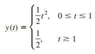
Although the two methods give the same result, as expected, notice
that it is more convenient to fold the unit step function u(t) than fold
g(t) in this example. Figure.(8) shows y(t).

Laplace Transform Convolution Integral Example 3
For the RL circuit in Figure.(9a), use the convolution integral to find the response io(t) due to the excitation shown in Figure.(9b).

This problem can be solved in two ways: directly using the convolution integral or using the graphical technique. To use either approach, we first need the unit impulse response h(t) of the circuit. In the s domain, applying the current division principle to the circuit in Figure.(10a) gives
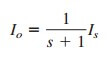 Hence,

and the inverse Laplace transform of this gives

Figure.(10b) shows the impulse response h(t) of the circuit.

METHOD 1 : To use the convolution integral directly, recall that the response is given in the s domain as
![]()
With the given is (t) in Figure.(9b),
![]()
so that

Since u(λ − 2) = 0 for 0 < λ < 2, the integrand involving u(λ) is nonzero for all λ > 0, whereas the integrand involving u(λ − 2) is nonzero only for λ > 2. The best way to handle the integral is to do the two parts separately.
For 0 < t < 2,

For t > 2,

Substituting Equations.(3.4) and (3.5) into (3.3) gives

METHOD 2 : To use the graphical technique, we may fold is(t) in Figure.(9a) and shift by t, as shown in Figure.(11a).

For 0 < t < 2, the overlap between
is(t − λ) and h(λ) is from 0 to t, so that

For t > 2, the two functions overlap between (t − 2) and t, as in Figure.(11b). Hence

From Equations.(3.7) and (3.8), the response is

which is the same as in Equation.(3.6). Thus, the response io(t) along the excitation is(t) is as shown in Figure.(12).